Chapter 4
Differential Relations for Fluid Flow
Differential Relations for Fluid Flow
Overview
In chapter four, the conservation equations on integral form derived in chapter 3 are applied to infinitesimal control volumes and the resulting relations are the conservation equations on partial differential form (continuity, momentum, and energy). The Navier-Stokes equations are introduced and flow rotation and vorticity is discussed. The partial differential flow equations are in general difficult to solve and numerical approaches are needed but analytical solutions exists for a few applications.
Roadmap
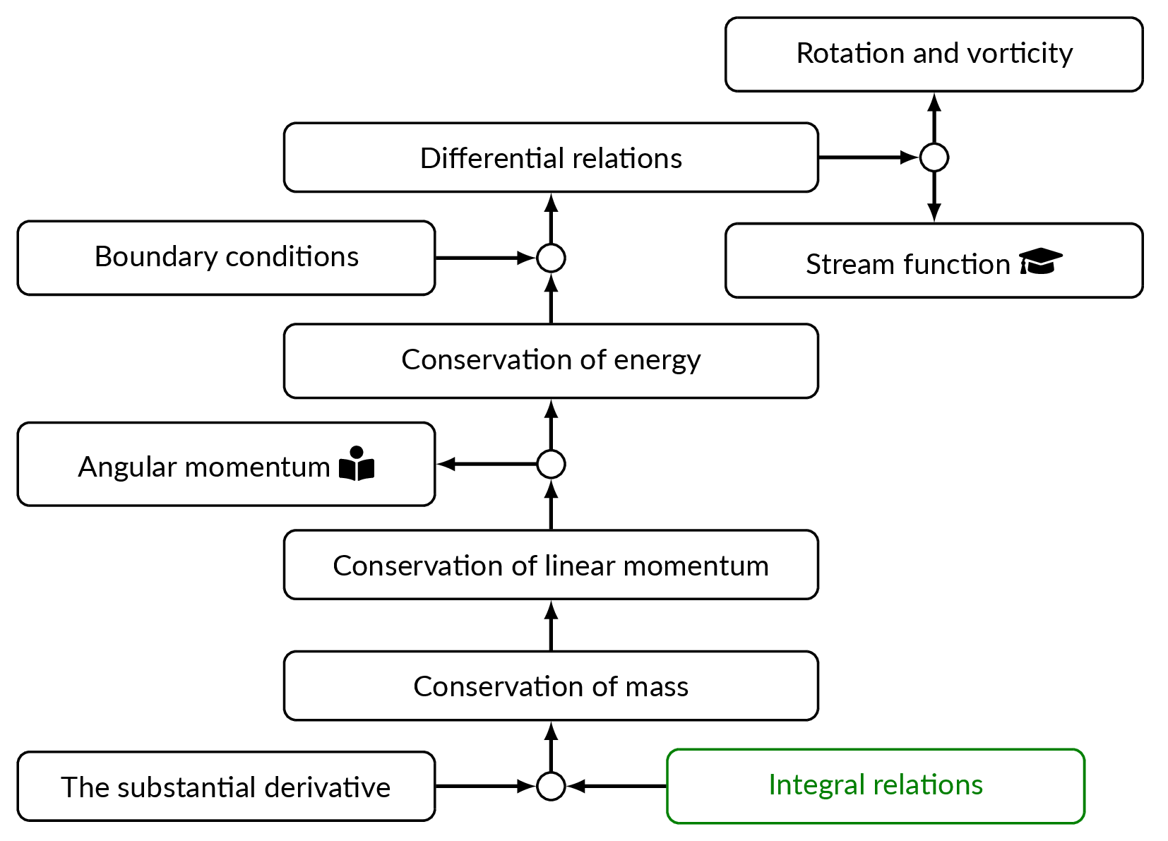
The Substantial Derivative
Acceleration of the flow in a point (\(x,y,z\)) is by definition obtained as
$$\mathbf{a}=\dfrac{d\mathbf{V}}{dt}=\mathbf{e}_x\dfrac{du}{dt}+\mathbf{e}_y\dfrac{dv}{dt}+\mathbf{e}_z\dfrac{dw}{dt}$$Each scalar component of the velocity vector (\(u,v,w\)) is a function of four variables (\(x,y,z,t\)) and thus
$$\dfrac{du(x,y,z,t)}{dt}=\dfrac{\partial u}{\partial t}+\dfrac{\partial u}{\partial x}{\color{MatlabB}{\dfrac{dx}{dt}}}+\dfrac{\partial u}{\partial y}{\color{MatlabA}{\dfrac{dy}{dt}}}+\dfrac{\partial u}{\partial z}{\color{MatlabE}{\dfrac{dz}{dt}}}$$By definition \(dx/dt=u\), \(dy/dt=v\), and \(dz/dt=w\)
$$\dfrac{du(x,y,z,t)}{dt}=\dfrac{\partial u}{\partial t}+u\dfrac{\partial u}{\partial x}+v\dfrac{\partial u}{\partial y}+w\dfrac{\partial u}{\partial z}=\dfrac{\partial u}{\partial t}+(\mathbf{V}\cdot\nabla)u$$$$\mathbf{a}=\underbrace{\dfrac{\partial \mathbf{V}}{\partial t}}_{local}+\underbrace{\left(u\dfrac{\partial \mathbf{V}}{\partial x}+v\dfrac{\partial \mathbf{V}}{\partial y}+w\dfrac{\partial \mathbf{V}}{\partial z}\right)}_{convective}=\dfrac{\partial \mathbf{V}}{\partial t}+(\mathbf{V}\cdot\nabla)\mathbf{V}=\dfrac{D\mathbf{V}}{Dt}$$
- local acceleration: only in unsteady flows
- convective acceleration: fluid particle that moves through regions of spatially varying velocity
The sum of the local derivative and the convective derivative is often referred to as the substantial derivative. The substantial derivative follows a fluid particle but is expressed in an Eulerian frame of reference. The substantial derivative is an operator that can be applied to any variable such as for example pressure
$$\dfrac{Dp}{Dt}=\dfrac{\partial p}{\partial t}+u\dfrac{\partial p}{\partial x}+v\dfrac{\partial p}{\partial y}+w\dfrac{\partial p}{\partial z}=\dfrac{\partial p}{\partial t}+(\mathbf{V}\cdot\nabla)p$$Conservation of Mass
The partial differential form of the continuity equation is obtained by applying the integral conservation of mass relation from chapter 3 to an infinitesimal control volume.

The result of the mass balance for the infinitesimal control volume reads
$$\dfrac{\partial \rho}{\partial t} + \dfrac{\partial}{\partial x}(\rho u) + \dfrac{\partial}{\partial y}(\rho v) + \dfrac{\partial}{\partial z}(\rho w) = 0$$or in more compact form using vector notation
$$\dfrac{\partial \rho}{\partial t} + \nabla \cdot (\rho \mathbf{V}) = 0$$Incompressible flow (constant density)
$$\dfrac{\partial u}{\partial x} + \dfrac{\partial v}{\partial y} + \dfrac{\partial w}{\partial z} = \nabla \cdot \mathbf{V} = 0$$Conservation of Linear Momentum
Applying the integral relation for conservation of linear momentum from chapter 3 to an infinitesimal control volume gives the following result
$$\sum \mathbf{F}=\left[\dfrac{\partial}{\partial t}(\mathbf{V}\rho) + \dfrac{\partial}{\partial x}(\rho u \mathbf{V}) + \dfrac{\partial}{\partial y}(\rho v \mathbf{V}) + \dfrac{\partial}{\partial z}(\rho w \mathbf{V})\right]dxdydz$$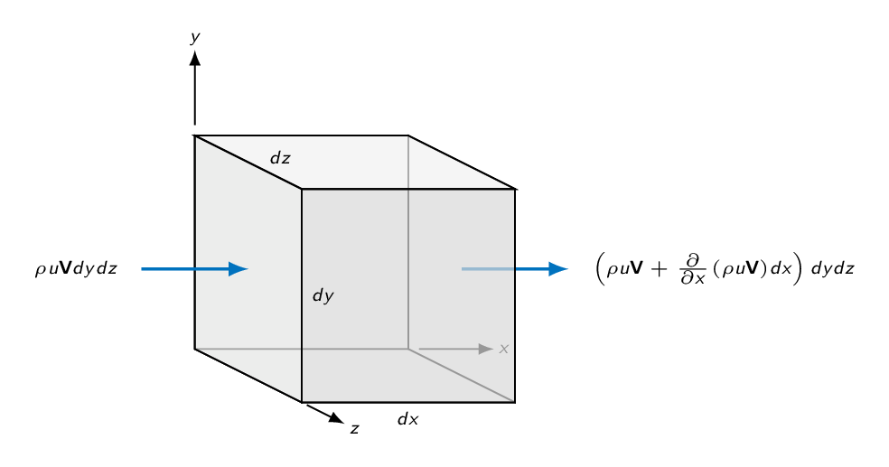
The derivatives may be rewritten as follows
$$ \underbrace{\dfrac{\partial}{\partial t}(\mathbf{V}\rho)}_{ \mathbf{V}\frac{\partial \rho}{\partial t}+ \rho\frac{\partial \mathbf{V}}{\partial t} } + \underbrace{\dfrac{\partial}{\partial x}(\rho u \mathbf{V})}_{ \mathbf{V}\frac{\partial}{\partial x}(\rho u)+ \rho u\frac{\partial \mathbf{V}}{\partial x} } + \underbrace{\dfrac{\partial}{\partial y}(\rho v \mathbf{V})}_{ \mathbf{V}\frac{\partial}{\partial y}(\rho v)+ \rho v\frac{\partial \mathbf{V}}{\partial y} } + \underbrace{\dfrac{\partial}{\partial z}(\rho w \mathbf{V})}_{ \mathbf{V}\frac{\partial}{\partial z}(\rho w)+ \rho w\frac{\partial \mathbf{V}}{\partial z} } $$If collecting terms after rewriting the derivatives as proposed above, the continuity equation is identified as part of the equation.
$$\mathbf{V}\underbrace{\left[\dfrac{\partial \rho}{\partial t} + \nabla \cdot (\rho \mathbf{V})\right]}_{the\ continuity\ equation} + \rho \underbrace{\left( \dfrac{\partial \mathbf{V}}{\partial t} + u\dfrac{\partial \mathbf{V}}{\partial x} + v\dfrac{\partial \mathbf{V}}{\partial y} + w\dfrac{\partial \mathbf{V}}{\partial z} \right)}_{\dfrac{\partial \mathbf{V}}{\partial t}+(\mathbf{V}\cdot\nabla)\mathbf{V}=\dfrac{D\mathbf{V}}{Dt}}$$and thus
$$\sum \mathbf{F} = {\color{MatlabA}{\rho \dfrac{D\mathbf{V}}{Dt}}}dxdydz$$The forces are body forces (gravity) and surface forces in the form of pressure forces and viscous forces. The surface forces (pressure and viscous stresses) are summarized in the stress tensor \(\sigma_{ij}\). For an arbitrary surface, pressure results in a force in the negative surface normal direction and thus pressure appears with a negative sign in the diagonal of the stress tensor.
$$ \sigma_{ij}=\left| \begin{array}{ccc} -p + \tau_{xx} & \tau_{yx} & \tau_{zx} \\ \tau_{xy} & -p + \tau_{yy} & \tau_{zy} \\ \tau_{xz} & \tau_{yz} & -p + \tau_{zz} \end{array} \right| $$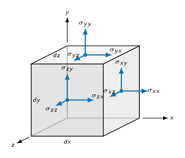
In the \(x\)-direction, we will get the following contribution from surface forces
$$dF_{x,surf}=\left[-\dfrac{\partial p}{\partial x}+\dfrac{\partial}{\partial x}(\tau_{xx})+\dfrac{\partial}{\partial y}(\tau_{yx})+\dfrac{\partial}{\partial z}(\tau_{zx})\right]dxdydz$$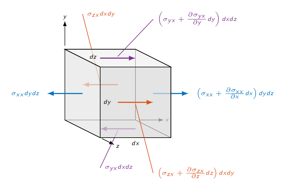
Adding the \(y\)- and \(z\)-direction forces we get
$$d\mathbf{F}=\left[-\nabla p+\nabla \cdot \tau_{ij}\right]dxdydz$$where
$$ \tau_{ij}=\left| \begin{array}{ccc} \tau_{xx} & \tau_{yx} & \tau_{zx} \\ \tau_{xy} & \tau_{yy} & \tau_{zy} \\ \tau_{xz} & \tau_{yz} & \tau_{zz} \end{array} \right| $$is the viscous stress tensor
Combining the forces on the infinitesimal control volume with the momentum balance for the same we get
$$\dfrac{\partial u}{\partial t} + u\dfrac{\partial u}{\partial x} + v\dfrac{\partial u}{\partial y} + w\dfrac{\partial u}{\partial z} = g_x - \dfrac{1}{\rho}\dfrac{\partial p}{\partial x} + \dfrac{1}{\rho}\left[\dfrac{\partial \tau_{xx}}{\partial x} + \dfrac{\partial \tau_{yx}}{\partial y} + \dfrac{\partial \tau_{zx}}{\partial z}\right]$$ $$\dfrac{\partial v}{\partial t} + u\dfrac{\partial v}{\partial x} + v\dfrac{\partial v}{\partial y} + w\dfrac{\partial v}{\partial z} = g_y - \dfrac{1}{\rho}\dfrac{\partial p}{\partial y} + \dfrac{1}{\rho}\left[\dfrac{\partial \tau_{xy}}{\partial x} + \dfrac{\partial \tau_{yy}}{\partial y} + \dfrac{\partial \tau_{zy}}{\partial z}\right]$$ $$\dfrac{\partial w}{\partial t} + u\dfrac{\partial w}{\partial x} + v\dfrac{\partial w}{\partial y} + w\dfrac{\partial w}{\partial z} = g_z - \dfrac{1}{\rho}\dfrac{\partial p}{\partial z} + \dfrac{1}{\rho}\left[\dfrac{\partial \tau_{xz}}{\partial x} + \dfrac{\partial \tau_{yz}}{\partial y} + \dfrac{\partial \tau_{zz}}{\partial z}\right]$$or in more compact vector form
$$\dfrac{D\mathbf{V}}{Dt} = \mathbf{g}-\dfrac{1}{\rho}\nabla p + \dfrac{1}{\rho}\nabla \cdot \tau_{ij}$$Recall
For a Newtonian fluid, the viscous stresses are proportional to the element strain and the viscosity
For incompressible flow:
$$\tau_{xx}=2\mu\dfrac{\partial u}{\partial x},\ \tau_{yy}=2\mu\dfrac{\partial v}{\partial y},\ \tau_{zz}=2\mu\dfrac{\partial w}{\partial z}$$ $$\tau_{xy}=\tau_{yx}=\mu\left(\dfrac{\partial u}{\partial y}+\dfrac{\partial v}{\partial x}\right),\ \tau_{xz}=\tau_{zx}=\mu\left(\dfrac{\partial u}{\partial z}+\dfrac{\partial w}{\partial x}\right)$$ $$\tau_{yz}=\tau_{zy}=\mu\left(\dfrac{\partial v}{\partial z}+\dfrac{\partial w}{\partial y}\right)$$Inserting the relations between stress components and velocity gradients we get the Navier-Stokes equations (here given in the form applicable for incompressible flows)
$$\rho \dfrac{Du}{Dt} = \rho g_x - \dfrac{\partial p}{\partial x} + \mu\left(\dfrac{\partial^2u}{\partial x^2} + \dfrac{\partial^2 u}{\partial y^2} + \dfrac{\partial^2 u}{\partial z^2}\right)$$ $$\rho \dfrac{Dv}{Dt} = \rho g_y - \dfrac{\partial p}{\partial y} + \mu\left(\dfrac{\partial^2v}{\partial x^2} + \dfrac{\partial^2 v}{\partial y^2} + \dfrac{\partial^2 v}{\partial z^2}\right)$$ $$\rho \dfrac{Dw}{Dt} = \rho g_z - \dfrac{\partial p}{\partial z} + \mu\left(\dfrac{\partial^2w}{\partial x^2} + \dfrac{\partial^2 w}{\partial y^2} + \dfrac{\partial^2 w}{\partial z^2}\right)$$
Conservation of Energy
To derive the energy equation on partial differential form, we again use the approach of applying the relation for conservation of energy on integral form from chapter 3 for an infinitesimal control volume. The resulting equation reads
$$\dot{Q}-\dot{W}_\nu=\left[ \frac{\partial}{\partial t}(\rho e) + \frac{\partial}{\partial x}(\rho u {\color{MatlabA}{h}}) + \frac{\partial}{\partial y}(\rho v {\color{MatlabA}{h}}) + \frac{\partial}{\partial z}(\rho w {\color{MatlabA}{h}})\right]dxdydz$$Using the chain rule for the derivatives on the right-hand-side, the relation above can be rewritten as
$$\dot{Q}-\dot{W}_\nu=\left[ \rho\frac{De}{Dt} + p\nabla\cdot\mathbf{V}+\mathbf{V}\cdot\nabla p \right]dxdydz$$Added Heat
According the Fourier's law of conduction, the heat flux is proportional to the temperature gradient
$$\mathbf{q}=-k\nabla T$$where \(k\) is the thermal conductivity and \(\mathbf{q}\) is heat transfer per unit area. A balance of heat flux over the infinitesimal control volume gives
$$\dot{Q}=-\left[ \frac{\partial q_x}{\partial x} + \frac{\partial q_y}{\partial y} + \frac{\partial q_z}{\partial z} \right]dxdydz = -\nabla \cdot \mathbf{q} dxdydz$$or
$$\dot{Q} = \nabla \cdot (k\nabla T) dxdydz$$
Viscous Work
The rate of work done by viscous stresses equals the product of the stress component, its corresponding velocity component and surface area
The viscous work contribution is obtained by performance a balance over the infinitesimal control volume.
$$\dot{W}_\nu = -\left[ \frac{\partial}{\partial x}(u\tau_{xx}+v\tau_{xy}+w\tau_{xz}) + \frac{\partial}{\partial y}(u\tau_{yx}+v\tau_{yy}+w\tau_{yz}) + \frac{\partial}{\partial z}(u\tau_{zx}+v\tau_{zy}+w\tau_{zz}) \right] dxdydz$$or
$$\dot{W}_\nu = -\nabla \cdot (\mathbf{V}\cdot\tau_{ij})dxdydz$$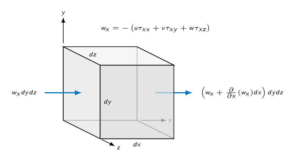
Inserting the expressions for heat addition and viscous work in the energy equation we get
$$ \nabla \cdot (k\nabla T) + \nabla \cdot (\mathbf{V}\cdot\tau_{ij}) = \rho\frac{De}{Dt} + p\nabla\cdot\mathbf{V}+\mathbf{V}\cdot\nabla p $$Finally, the shear stress terms are rewritten by introducing viscous dissipation
$$ \nabla \cdot (\mathbf{V}\cdot\tau_{ij}) = \mathbf{V} \cdot (\nabla\cdot\tau_{ij}) + \phi $$where
$$ \phi = \mu\left[ 2\left(\frac{\partial u}{\partial x}\right)^2 + 2\left(\frac{\partial v}{\partial y}\right)^2 + 2\left(\frac{\partial w}{\partial z}\right)^2 + \left(\frac{\partial v}{\partial x}+\frac{\partial u}{\partial y}\right)^2 + \left(\frac{\partial w}{\partial y} +\frac{\partial v}{\partial z}\right)^2 + \left(\frac{\partial u}{\partial z}+\frac{\partial w}{\partial x}\right)^2\right] $$All terms in the viscous-dissipation function are quadratic which means that in a viscous flow there will always be losses, which is in line with the second law of thermodynamics
Writing out the energy \(e\) as the sum of internal energy, kinetic energy per unit mass, and potential energy per unit mass, the energy equation (after some manipulation) reads
$$\rho \frac{D\hat{u}}{Dt} + p \nabla \cdot \mathbf{V} = \nabla\cdot(k\nabla T) + \phi$$Local and convective changes of internal energy are balanced by pressure work, heat addition and viscous dissipation - viscous dissipation will always increase the internal energy of the fluid
Rotation and Vorticity
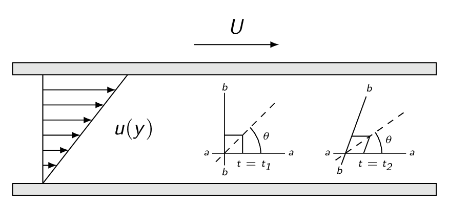
Is the Couette flow in the figure below irrotational? It sure looks like it is but the change in bisector angle for a fluid element reveals that the flow is in fact rotational.
The bisector angle for the fluid element in the figure below is obtained as
$$\beta=\frac{\pi}{2}+\theta_B-\theta_A$$ $$\theta=\frac{\beta}{2}+\theta_A=\frac{\pi}{4}+\frac{1}{2}(\theta_A+\theta_B)$$and thus the angular velocity of the bisector is given by
$$\dot\theta=\frac{1}{2}\left(\dot\theta_A+\dot\theta_B\right)$$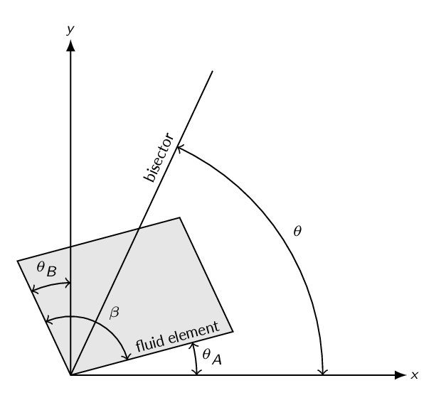 $$\sin (\Delta \theta_A)=\frac{\Delta y_1}{\Delta x}\approx\frac{\left(v+\frac{\partial v}{\partial x}\Delta x\right)\Delta t -v\Delta t}{\Delta x}=\frac{\partial v}{\partial x}\Delta t$$
\(\sin(\Delta \theta_A)\approx \Delta \theta_A\) for small angles, which means that
$$\underbrace{\frac{\Delta \theta_A}{\Delta t}}_{=\dot\theta_A}\approx\frac{\partial v}{\partial x}$$In the same way \(\dot\theta_B\approx-\frac{\partial u}{\partial y}\) and the angular velocity of the bisector for a fluid element can now be expressed as
$$\dot\theta=\frac{1}{2}\left(\dot\theta_A+\dot\theta_B\right)=\frac{1}{2}\left(\frac{\partial v}{\partial x}-\frac{\partial u}{\partial y}\right)$$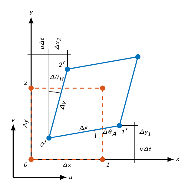
In the same way we can get the angular velocities in all coordinate directions
$$\omega_z=\frac{1}{2}\left(\frac{\partial v}{\partial x}-\frac{\partial u}{\partial y}\right)$$ $$\omega_x=\frac{1}{2}\left(\frac{\partial w}{\partial y}-\frac{\partial v}{\partial z}\right)$$ $$\omega_y=\frac{1}{2}\left(\frac{\partial u}{\partial z}-\frac{\partial w}{\partial x}\right)$$or
$$ \mathbf{\omega}=\frac{1}{2}\left| \begin{array}{ccc} \mathbf{e}_x & \mathbf{e}_y & \mathbf{e}_z \\[5pt] \frac{\partial}{\partial x} & \frac{\partial}{\partial y} & \frac{\partial}{\partial z}\\[5pt] u & v & w \end{array} \right| =\frac{1}{2}curl(\mathbf{V}) $$Flow vorticity is defined as \(\zeta=2\omega\)
Study Guide
The questions below are intended as a "study guide" and may be helpful when reading the text book.
- What is the difference between the control volume in an integral formulation and a differential formulation of the governing equations?
- Rewrite the acceleration using the chain rule and group the terms into local acceleration terms and convective acceleration terms
- Explain the physical meaning of the local acceleration term and the convective acceleration term
- The continuity equation on differential form:
- Derive the continuity equation on differential form starting from the integral form for a fixed control volume $$\int_{cv}\dfrac{\partial \rho}{\partial t}d\mathcal{V}+\sum_i\left(\rho_iA_iV_i\right)_{out}-\sum_i\left(\rho_iA_iV_i\right)_{in}=0$$ and let the size of the control volume reduce to infinitesimal size
- How can we simplify the continuity equation on differential form under the following circumstances?
$$\dfrac{\partial \rho}{\partial t}+\dfrac{\partial (\rho u)}{\partial x}+\dfrac{\partial (\rho v)}{\partial y}+\dfrac{\partial (\rho w)}{\partial z}=0$$
- steady-state flow
- incompressible flow
- The momentum equation on differential form:
- Derive the momentum equation on differential form starting from the integral form $$\sum\mathbf{F}=\dfrac{d}{dt}\left(\int_{cv}\mathbf{V}\rho d\mathcal{V}\right)+\sum\left(\dot{m}_i\mathbf{V}_i\right)_{out}-\sum\left(\dot{m}_i\mathbf{V}_i\right)_{in}$$ and let the size of the control volume reduce to infinitesimal size
- A fluid element is subjected to both body forces and surface forces. Give an example of a body force and name the two surface forces.
- Make a sketch of a control volume used for the derivation of the governing equations on differential form and indicate the stresses acting on the surfaces of the cube in one selected direction. Write down the resulting surface force in the selected direction.
- What generates the stresses denoted \(\tau_{ij}\). What is the difference between \(\tau_{ij}\) and \(\sigma_{ij}\).
- The \(x\)-component of the Navier-Sokes equations reads: $$\dfrac{\partial u}{\partial t}+u\dfrac{\partial u}{\partial x}+v\dfrac{\partial u}{\partial y}+w\dfrac{\partial u}{\partial z}=g_x-\dfrac{1}{\rho}\dfrac{\partial p}{\partial x}+\dfrac{\mu}{\rho}\left(\dfrac{\partial^2 u}{\partial x^2}+\dfrac{\partial^2 u}{\partial y^2}+\dfrac{\partial^2 u}{\partial z^2}\right)$$ What is the physical meaning of each of the terms in the equation?
- Under what circumstances can the general formulation of the momentum equation be reduced to the Navier-Stokes equation?
- If the integral angular momentum equation is applied to a control volume and the control volume is reduced to infinitesimal size, one will see a special feature of the stress tensor \(\tau_{ij}\). What feature is that?
- What is the physical meaning of the terms in the simplified energy equation? $$\rho C_v\dfrac{dT}{dt}=k\nabla^2T+\Phi$$
- Simplify the following system of equations for incompressible flow. Use the relation between the stress tensor and velocity derivatives applicable for Newtonian fluids. $$\dfrac{\partial \rho}{\partial t}+\nabla\cdot\left(\rho \mathbf{V}\right)=0$$ $$\rho\dfrac{d\mathbf{V}}{dt}=\rho \mathbf{g}-\nabla p+\nabla\cdot \tau_{ij}$$ $$\rho \dfrac{d \hat{u}}{dt}+p\left(\nabla\cdot\mathbf{V}\right)=\nabla\cdot\left(k\nabla T\right)+\Phi$$ What unknown properties can be calculated and how many equations do we have?
- What boundary conditions are often used for velocity and temperature at a solid wall?
- 2D incompressible duct flow:
- Simplify the continuity equation and Navier-Stokes equations without pressure gradient driven by a moving upper wall, i.e., Couette flows.
- Simplify the continuity equation and Navier-Stokes equations for pressure-driven flow, i.e., Poiseuille flows.
- Show that the Couette flow is rotational by analyzing a small fluid element.
- How is vorticity defined?
| Document Archive | ||
| MTF053_C04.pdf | Lecture notes chapter 4 | |
| MTF053_Formulas-Tables-and-Graphs.pdf | A collection of formulas, tables, and graphs | |
| MTF053_Study-Guide.pdf | A collection of theory questions that give a good representation of the theory covered in the course | |