Chapter 3
Integral Relations for a Control Volume
Integral Relations for a Control Volume
Overview
In this chapter, we will start to investigate fluid flows. Reynolds transport theorem, a tool that converts relations for a system to relations for a control volume, is introduced. Reynolds transport theorem is used to derive conservation relations on integral form (for a control volume). The relations derived are; conservation of mass, conservation of linear momentum, conservation of angular momentum, and conservation of energy. The relation for conservation of linear momentum forms the basis for the famous Bernoulli equation that is also introduced in this chapter.
Roadmap
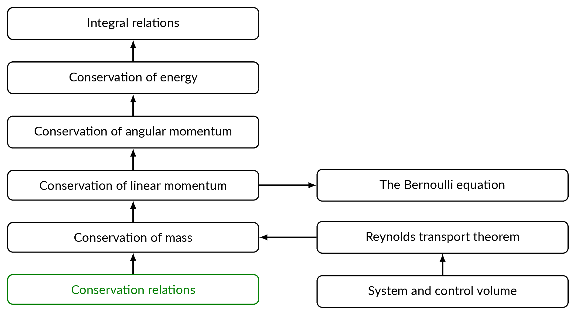
System and Control Volume
All laws of mechanics are derived for a system. A system is an arbitrary quantity of mass of fixed identity \(m\) that is separated from its surroundings by its boundaries. Physical relations describes the interaction between the system and its surroundings. In chapter 3, conservation relations for fluid flows are derived with the starting point in the following conservation laws for a system
- Conservation of mass
- Conservation of linear momentum
- Conservation of angular momentum
- Conservation of energy
Mass flow through a control volume
The mass flow through a control volume is calculated by integrating the fluid density times the scalar product of the velocity vector and the surface normal over the control volume surface. Only the velocity component that is parallel with the surface normal will contribute to the net flux of mass over the control volume surface as shown in the figure below.
$$\dot{m}=\int_{\partial \Omega}\rho(\mathbf{V}\cdot\mathbf{n})dA$$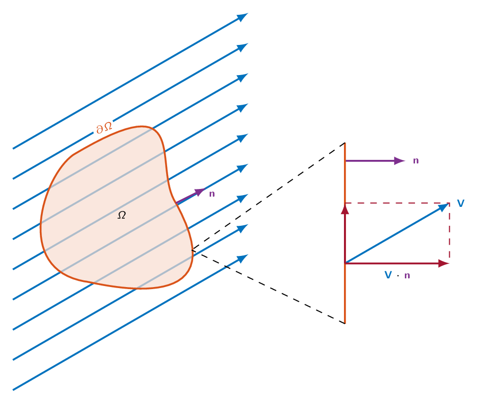
Reynolds Transport Theorem
Reynolds transport theorem is a tool to rewrite relations for a system to relations for a control volume, which is exactly what this chapter is about. Let \(B\) be any extensive property of the fluid (energy, momentum, enthalpy, ... ). \(\beta\) is the corresponding intensive value (the amount \(B\) per unit mass).
The total amount of \(B\) in the control volume is obtained by integrating over the control volume
$$B_{CV}=\int_{CV}\beta dm=\int_{CV}\beta \rho d\mathcal{V}$$where \(\beta=\dfrac{dB}{dm}\)
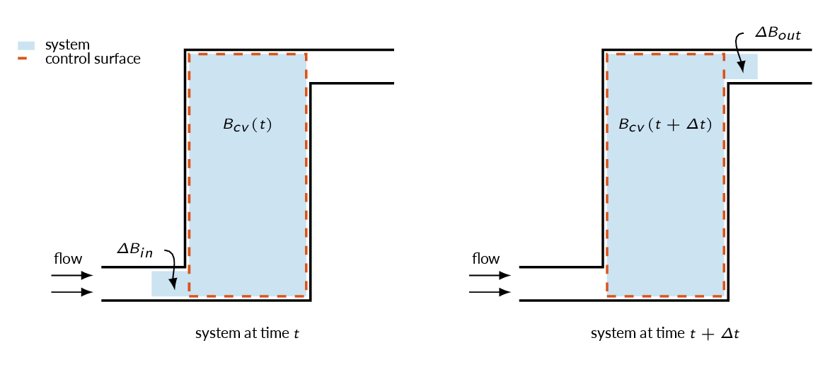 $$B_{sys}(t)=B_{cv}(t)+\Delta B_{in}$$
$$B_{sys}(t+\Delta t)=B_{cv}(t+\Delta t)+\Delta B_{out}$$
$$B_{sys}(t)=B_{cv}(t)+\Delta B_{in}$$
$$B_{sys}(t+\Delta t)=B_{cv}(t+\Delta t)+\Delta B_{out}$$
Rate of change of \(B\) within the control volume
$$\frac{d}{dt}\left(\int_{CV}\beta\rho d\mathcal{V}\right)$$Net flux of \(B\) over the control volume surface
$$\int_{CS}\beta \rho (\mathbf{V}\cdot\mathbf{n})dA$$Reynolds transport theorem
$$\underbrace{\frac{d}{dt}(B_{sys})}_{Lagrange}=\underbrace{\frac{d}{dt}\left(\int_{CV}\beta\rho d\mathcal{V}\right)+\int_{CS}\beta \rho (\mathbf{V}\cdot\mathbf{n})dA}_{Euler}$$For a fixed control volume (the volume does not change in time)
$$\frac{d}{dt}\left(\int_{CV}\beta\rho d\mathcal{V}\right) = \int_{CV}\frac{\partial}{\partial t}(\beta\rho) d\mathcal{V}$$If the control volume moves with the constant velocity \(\mathbf{V_s}\), the relative velocity of the fluid crossing the control volume surface \(\mathbf{V_r}\) is
$$\mathbf{V_r}=\mathbf{V}-\mathbf{V_s}$$and thus
$$\frac{d}{dt}(B_{sys})=\frac{d}{dt}\left(\int_{CV}\beta\rho d\mathcal{V}\right)+\int_{CS}\beta \rho (\mathbf{V_r}\cdot\mathbf{n})dA$$Conservation of Mass
Reynolds transport theorem with \(B=m\) and \(\beta=dB/dm=dm/dm=1\)
$$\frac{d}{dt}(m_{sys})=0=\frac{d}{dt}\left(\int_{CV}\rho d\mathcal{V}\right)+\int_{CS}\rho (\mathbf{V_r}\cdot\mathbf{n})dA$$for a fixed control volume
$$\int_{CV}\frac{\partial \rho}{\partial t} d\mathcal{V}+\int_{CS}\rho (\mathbf{V_r}\cdot\mathbf{n})dA=0$$for a control volume with a number of one-dimensional inlets and outlets
$$\int_{CV}\frac{\partial \rho}{\partial t} d\mathcal{V}+\sum_i(\rho_i A_i V_i)_{out} - \sum_i(\rho_i A_i V_i)_{in} =0$$
Steady state \(\Rightarrow \partial \rho/\partial t = 0 \)
$$\int_{CS}\rho (\mathbf{V_r}\cdot\mathbf{n})dA=0$$or
$$\sum_i(\rho_i A_i V_i)_{out} = \sum_i(\rho_i A_i V_i)_{in}$$Incompressible flow \(\Rightarrow \partial \rho/\partial t = 0 \) $$\int_{CS}(\mathbf{V_r}\cdot\mathbf{n})dA=0$$
or
$$\sum_i(A_i V_i)_{out} = \sum_i(A_i V_i)_{in} $$Conservation of Linear Momentum
Reynolds transport theorem with \(B=m\mathbf{V}\) and \(\beta=dB/dm=d(m\mathbf{V})/dm=\mathbf{V}\)
$$\frac{d}{dt}(m\mathbf{V})_{sys}=\sum \mathbf{F}=\frac{d}{dt}\left(\int_{CV}\mathbf{V}\rho d\mathcal{V}\right)+\int_{CS}\mathbf{V}\rho (\mathbf{V_r}\cdot\mathbf{n})dA$$\(\mathbf{V}\) is the velocity relative to an inertial (non-accelerating) coordinate system. \(\sum \mathbf{F}\) is the vector sum of all forces on the system (surface forces and body forces). The relation is a vector relation (three components)
Forces: Solid bodies that protrude through the control volume surface and forces due to pressure and viscous stresses of the surrounding fluid.
Pressure forces
$$\mathbf{F}_{p}=\int_{CS}p(-\mathbf{n})dA$$ $$\mathbf{F}_{p}=\int_{CS}(p-p_{atm})(-\mathbf{n})dA=\int_{CS}p_{gage}(-\mathbf{n})dA$$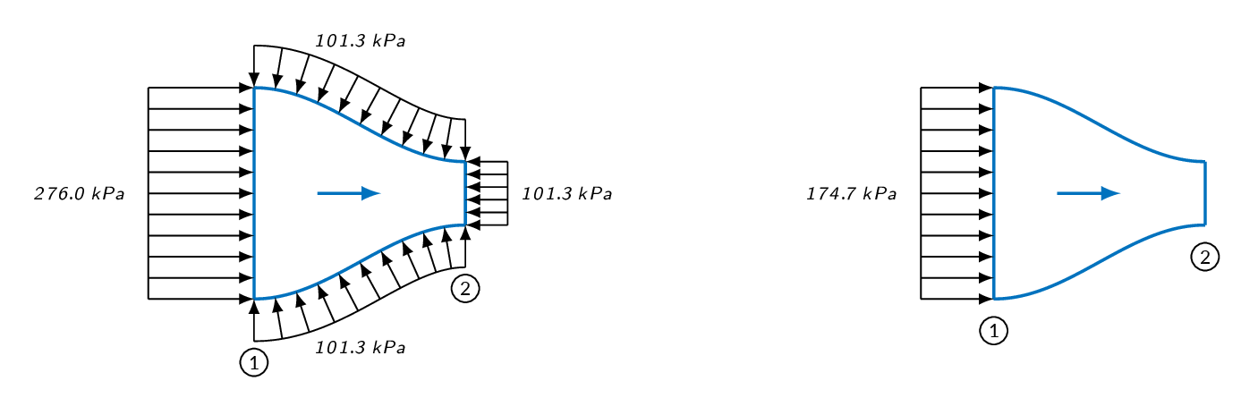
The Bernoulli Equation
The relation between pressure, velocity, and elevation in a frictionless flow
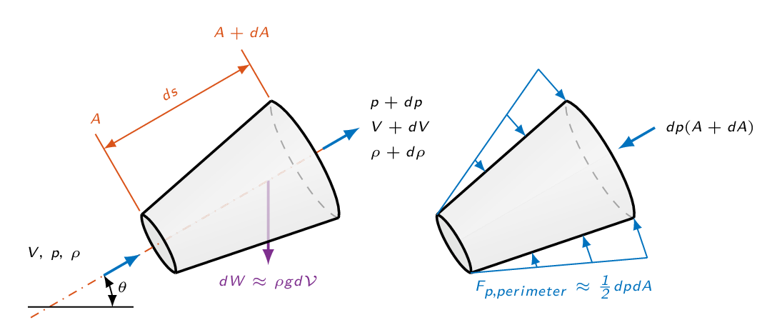
Bernoulli's equation for unsteady frictionless flow along a streamline (the relation just derived) can be integrated between any two points along the streamline
$$\int_1^2\frac{\partial V}{\partial t}ds+\int_1^2\frac{dp}{\rho}+\frac{1}{2}\left(V_2^2-V_1^2\right)+g\left(z_2-z_1\right)=0$$Steady (\(\partial V/\partial t = 0\)), incompressible (constant density) flow:
$$p_1+\frac{1}{2}\rho V_1^2+\rho g z_1=p_2+\frac{1}{2}\rho V_2^2+\rho g z_2=const$$Note! the following restrictive assumptions have been made in the derivation
- steady flow
many flows can be treated as steady at least when doing control volume type of analysis - incompressible flow
low velocity gas flow without significant changes in pressure, liquid flow - frictionless flow
friction is in general important - flow along a single streamline
different streamlines in general have different constants, we shall see later that under specific circumstances all streamlines have the same constant
In many flows, elevation changes are negligible
$$p_1+\frac{1}{2}\rho V_1^2=p_2+\frac{1}{2}\rho V_2^2=p_o$$- Static pressure: \(p_1\) and \(p_2\)
- Dynamic pressure: \(\frac{1}{2}\rho V_1^2\) and \(\frac{1}{2}\rho V_2^2\)
- Stagnation (total) pressure: \(p_o\)
The Bernoulli equation is the basis for velocity measurements using a Prandtl tube (see figure below).
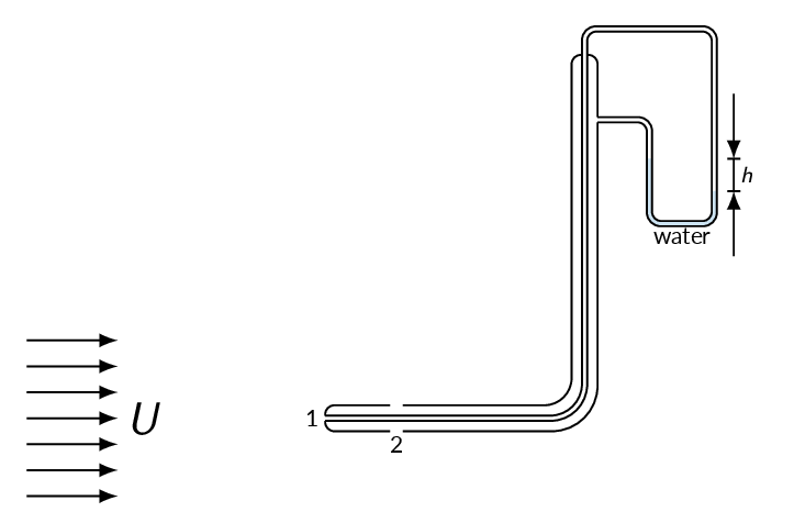 $$p_1+\frac{1}{2}\rho_{air}U_1^2+\rho g z_1=p_2+\frac{1}{2}\rho_{air}U_2^2+\rho g z_2$$
$$\left. \begin{array}{ll} U_1 & = 0.\\ U_2 & = U\\ z_1 & \approx z_2\\ p_1-p_2 & = \rho_{water}gh \end{array} \right\}\Rightarrow U = \sqrt{\frac{2\rho_{water}gh}{\rho_{air}}} $$
Conservation of Angular Momentum
Angular momentum about a point \(o\)
$$\mathbf{H}_o=\int_{syst}(\mathbf{r}\times\mathbf{V})dm=B$$where \(\mathbf{r}\) is the position vector from \(o\) to the element mass \(dm\) and \(\mathbf{V}\) is the velocity of that element
The amount of angular momentum per unit mass
$$\beta=\frac{d\mathbf{H}_o}{dm}=\mathbf{r}\times\mathbf{V}$$Reynold's transport theorem:
$$\left.\frac{d\mathbf{H}_o}{dt}\right |_{syst}=\frac{d}{dt}\left[\int_{CV}(\mathbf{r}\times\mathbf{V})\rho d\mathcal{V}\right]+\int_{CS}(\mathbf{r}\times\mathbf{V})\rho(\mathbf{V}_r\cdot\mathbf{n})dA$$Conservation of Energy
Reynold's transport theorem applied the the first law of thermodynamics (\(B=E,\ \beta=dE/dm=e\))
$$\frac{dQ}{dt}-\frac{dW}{dt}=\frac{dE}{dt}=\frac{d}{dt}\left(\int_{CV}e\rho d\mathcal{V}\right)+\int_{CS}e\rho (\mathbf{V}\cdot\mathbf{n})dA$$- positive \(Q\) - heat added to the system
- positive \(W\) - work done by the system on its surroundings
\(e_{other}\) could be related to, for example, chemical reactions, nuclear reactions, or magnetic fields and will not be considered here
$$e=\hat{u}+\frac{1}{2}V^2+gz$$The work term \(\dot{W}\) can be divided into shaft work, pressure work, and work related to viscous forces
$$\dot{W}=\dot{W}_s+\dot{W}_p+\dot{W}_\nu$$ $$\dot{W}_p=\int_{CS}p(\mathbf{V}\cdot\mathbf{n})dA$$ $$\dot{W}_\nu=-\int_{CS}\tau\cdot\mathbf{V}dA$$ $$\dot{Q}-\dot{W}_s-\dot{W}_\nu=\frac{d}{dt}\left(\int_{CV}e\rho d\mathcal{V}\right)+\int_{CS}\left(e+\frac{p}{\rho}\right)\rho (\mathbf{V}\cdot\mathbf{n})dA$$or
$$\dot{Q}-\dot{W}_s-\dot{W}_\nu=\frac{d}{dt}\left[\int_{CV}\left( \hat{u}+\frac{1}{2}V^2+gz \right)\rho d\mathcal{V}\right]+\int_{CS}\left(\hat{h}+\frac{1}{2}V^2+gz\right)\rho (\mathbf{V}\cdot\mathbf{n})dA$$where \(\hat{h}\) is the enthalpy defined as \(\hat{h}=\hat{u}+p/\rho\)
$$\left(\frac{p_1}{\rho g}+\frac{V_1^2}{2g}+z_1\right)_{in}=\left(\frac{p_2}{\rho g}+\frac{V_2^2}{2g}+z_2\right)_{out}+h_f-h_p+h_t$$Introducing the correction factor \(\alpha\)
$$\int\frac{1}{2}V^2\rho(\mathbf{V}\cdot\mathbf{n})dA=\frac{\alpha V_{av}^2}{2}\dot{m}$$where (for incompressible flow)
$$V_{av}=\frac{1}{A}\int udA$$$$\left(\frac{p_1}{\rho g}+\frac{\alpha_1 V_1^2}{2g}+z_1\right)_{in}=\left(\frac{p_2}{\rho g}+\frac{\alpha_2 V_2^2}{2g}+z_2\right)_{out}+h_f-h_p+h_t$$
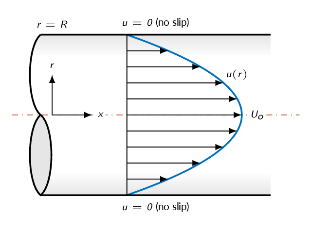
Laminar pipe flow
$$u(r)=U_{max}\left[1-\left(\frac{r}{R}\right)^2\right]$$which gives \(V_{av}=\frac{1}{2}U_{max}\) and \(\alpha=2.0\). For turbulent flows, \(\alpha=1\) is often a good assumption.
Study Guide
The questions below are intended as a "study guide" and may be helpful when reading the text book.
- Rewrite Newton's second law using the momentum of a system. What is the name of this relation?
- Define the angular momentum of a system
- Volume flow and mass flow:
- Show how the volume flow \(Q\) and mass flow \(\dot{m}\) over a control volume surface can be calculated in a general way
- How are volume flow \(Q\) and mass flow \(\dot{m}\) related if the density is constant
- How is the volume-averaged mean velocity over a surface defined for a fluid with constant density?
- Give examples of when it is appropriate to use fixed control volume, moving control volume, and deformable control volume, respectively.
- Reynolds transport theorem:
- In Reynolds transport theorem, \(B\) and \(\beta\) denotes extensive and intensive properties respectively. Explain the difference between \(B\) and \(\beta\).
- If an intensive property, \(\beta\), is known, how is the corresponding extensive property, \(B\), calculated?
- Give two examples of intensive and extensive properties
- Explain the physical meaning of each of the terms in Reynolds transport theorem: $$\dfrac{d}{dt}\left(B_{syst}\right)=\dfrac{d}{dt}\left(\int_{cv}\beta \rho d\mathcal{V}\right)+\int_{cs}\beta \rho \left(\mathbf{V}_r\cdot \mathbf{n}\right)dA$$
- How can the generic form of Reynolds transport theorem (above) be be simplified for a fix control volume?
- What does it mean that inlets and outlets are one-dimensional?
- How can we simplify Reynolds transport theorem for one-dimensional inlets and outlets?
- The continuity equation:
- Derive the continuity equation on integral form for a fixed control volume using Reynolds transport theorem
- Explain the physical meaning of each of the terms in the continuity equation on integral form
- How can we simplify the continuity equation on integral form under the following circumstances (assuming that the control volume is fixed)?
$$\int_{cv}\dfrac{\partial \rho}{\partial t}d\mathcal{V}+\int_{cs}\rho\left(\mathbf{V}\cdot\mathbf{n}\right)dA$$
- inlets and outlets can be assumed to be one-dimensional
- steady-state flow
- incompressible unsteady flow
- The momentum equation:
- Derive the momentum equation on integral form starting from Reynolds transport theorem
- Explain the physical meaning of each of the terms in the momentum equation on integral form
- How can we simplify the momentum equation on integral form under the following circumstances?
$$\dfrac{d}{dt}\left(m\mathbf{V}\right)_{syst}=\sum\mathbf{F}=\dfrac{d}{dt}\left(\int_{cv}\mathbf{V}\rho d\mathcal{V}\right)+\int_{cs}\mathbf{V}\rho\left(\mathbf{V}_r\cdot\mathbf{n}\right)dA$$
- fixed control volume
- fixed control volume and one-dimensional inlets and outlets
- fixed control volume, one-dimensional inlets and outlets, and steady-state flow
- What is gauge pressure?
- The Bernoulli equation:
- Derive the Bernoulli equation for steady-state, incompressible flow along a streamline $$\dfrac{p_1}{\rho}+\dfrac{1}{2}V_1^2+gz_1=\dfrac{p_2}{\rho}+\dfrac{1}{2}V_2^2+gz_2=const$$
- What assumptions are made in the derivation of the Bernoulli equation?
- The energy equation:
- What does \(Q\) and \(W\) in the energy equation represent?
- The energy per unit mass, \(e\), and the work are both divided into parts, what parts are the terms divided into?
- The Bernoulli equation is a simplified form of the energy equation. $$\dfrac{p_1}{\rho}+\dfrac{1}{2}V_1^2+gz_1=\dfrac{p_2}{\rho}+\dfrac{1}{2}V_2^2+gz_2=const$$ In what ways are the Bernoulli equation above more limited than the energy equation on the form given below? $$\left(\dfrac{p_1}{\gamma}+\dfrac{V_1^2}{2g}+z_1\right)=\left(\dfrac{p_2}{\gamma}+\dfrac{V_2^2}{2g}+z_2\right)+\dfrac{\hat{u}_2-\hat{u}_1-q}{g}$$
- Why is the kinetic energy correction factor introduced?
- Show that the kinetic energy correction factor is \(\alpha=2.0\) for laminar, incompressible pipe flow.
- Explain how to measure velocity using a Prandtl tube (Pitot-static tube) and derive the relation needed to estimate the velocity
- Explain how a venturi meter works and derive the relation needed to estimate the velocity
| Document Archive | ||
| MTF053_C03.pdf | Lecture notes chapter 3 | |
| MTF053_Formulas-Tables-and-Graphs.pdf | A collection of formulas, tables, and graphs | |
| MTF053_Study-Guide.pdf | A collection of theory questions that give a good representation of the theory covered in the course | |