Chapter 7
Flow Past Immersed Bodies
Flow Past Immersed Bodies
Overview
In this chapter theory for the analysis of external boundary-layer flows is derived. The boundary-layer equations are derived, which forms the basis for Blasius boundary layer theory for laminar boundary layers over flat plates. Prandtl's power law is used for turbulent boundary layers. For both laminar and turbulent boundary layers, estimates of boundary-boundary layer thickness, momentum thickness, displacement thickness, wall-shear stress (skin friction coefficient), and viscous drag are established. Lift and drag for bodies immersed in flows are discussed.
Roadmap
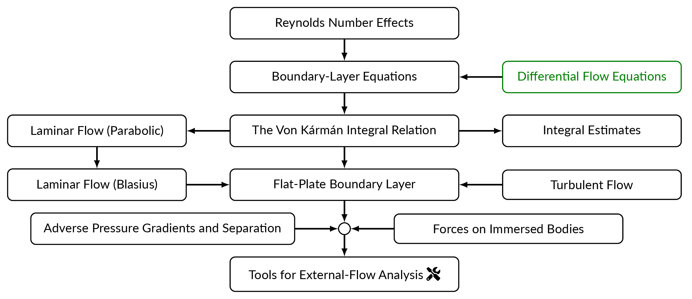
Boundary-Layer Equations
The boundary-layer equations are derived by performing a comparative order-of-magnitude analysis of the individual terms in the governing flow equations. The starting point is the non-dimensional, steady-state, incompressible flow equations on differential form.
$$\frac{\partial u^\ast}{\partial x^\ast}+\frac{\partial v^\ast}{\partial y^\ast}=0$$ $$u^\ast\frac{\partial u^\ast}{\partial x^\ast}+v^\ast\frac{\partial u^\ast}{\partial y^\ast}=-\frac{\partial p^\ast}{\partial x^\ast}+\frac{1}{Re}\left(\frac{\partial^2 u^\ast}{\partial {x^\ast}^2}+\frac{\partial^2 u^\ast}{\partial {y^\ast}^2}\right)$$ $$u^\ast\frac{\partial v^\ast}{\partial x^\ast}+v^\ast\frac{\partial v^\ast}{\partial y^\ast}=-\frac{\partial p^\ast}{\partial y^\ast}+\frac{1}{Re}\left(\frac{\partial^2 v^\ast}{\partial {x^\ast}^2}+\frac{\partial^2 v^\ast}{\partial {y^\ast}^2}\right)$$where stars means non-dimensional. The variables in the equations are made non-dimensional as follows:
$$x^\ast=x/L,\ y^\ast=y/L,\ u^\ast=u/U,\ v^\ast=v/U,\ p^\ast=p/(\rho U^2)$$where \(L\) and \(U\) are representative length and velocity scales. For a boundary layer over a flat plate \(L\) is the length of the plate and \(U\) is the freestream velocity. The Reynolds number appearing in the momentum equations is defined as
$$Re=\frac{UL}{\nu}$$To be able to find the relative sizes of different terms in the equations, we will first have a look at some of the flow parameters and operators
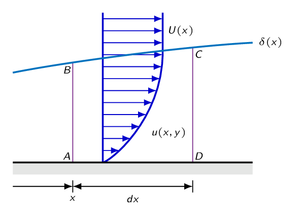
$$u^\ast=u/U\sim 1\ x^\ast=x/L\sim 1,\ y^\ast=y/L\sim \delta^\ast$$where \(\delta\) denotes boundary layer thickness and \(\delta^\ast=\delta/L\). Now the relative sizes of some of the variables are defined but what about the derivatives? Let's try to get an estimate of the derivatives of \(u\) in the wall-normal direction using the figure below. \(u^\ast\) is 0 at the wall and \(u^\ast\rightarrow 1\) as \(y \rightarrow \delta\).
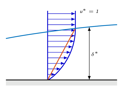 $$\frac{\partial u^\ast}{\partial y^\ast}\sim\frac{1-0}{\delta^\ast}=\frac{1}{\delta^\ast}$$
\(\partial u^\ast/\partial y^\ast \sim 1/\delta^\ast\) at the wall and \(\partial u^\ast/\partial y^\ast\rightarrow 0\) as \(y \rightarrow \delta\).
$$\frac{\partial^2 u^\ast}{\partial {y^\ast}^2}=\frac{\partial}{\partial y^\ast}\frac{\partial u^\ast}{\partial y^\ast}\sim\frac{\left|0-1/\delta^\ast\right|}{\delta^\ast}=\frac{1}{\delta^{\ast^2}}$$
$$\frac{\partial u^\ast}{\partial y^\ast}\sim\frac{1-0}{\delta^\ast}=\frac{1}{\delta^\ast}$$
\(\partial u^\ast/\partial y^\ast \sim 1/\delta^\ast\) at the wall and \(\partial u^\ast/\partial y^\ast\rightarrow 0\) as \(y \rightarrow \delta\).
$$\frac{\partial^2 u^\ast}{\partial {y^\ast}^2}=\frac{\partial}{\partial y^\ast}\frac{\partial u^\ast}{\partial y^\ast}\sim\frac{\left|0-1/\delta^\ast\right|}{\delta^\ast}=\frac{1}{\delta^{\ast^2}}$$
Note! The sign of terms is not important here, we are only interested in the order of magnitude
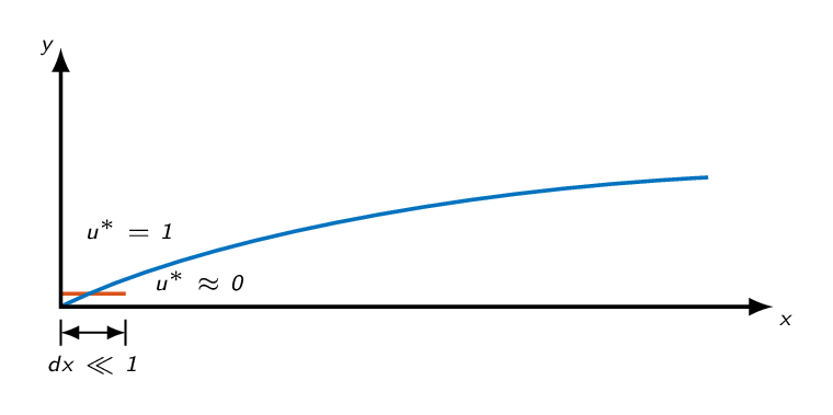
Now, let's have a look at the derivatives of \(u\) in the \(x\)-direction. Again we will make use of a schematic representation of the boundary layer given by the figure below. To get an estimate of the size of the derivatives, we will see how variables changes as we follow a horizontal line cutting through the boundary layer. The vertical position of the line is a bit above the wall, which means the at \(x=0\), the line is outside of the boundary layer. As the boundary layer grows downstream, the line gets, in relative terms, closer and closer to the wall. By looking at the development of \(u\) as \(x\) approaches the length of the plate, we can estimate the relative magnitude of the derivatives of \(u\) in the \(x\)-direction.
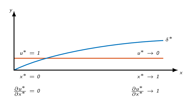 $$\frac{\partial u^\ast}{\partial x^\ast}\sim\frac{\left|0-1\right|}{1-0}=1$$
$$\frac{\partial^2 u^\ast}{\partial {x^\ast}^2}=\frac{\partial}{\partial x^\ast}\frac{\partial u^\ast}{\partial x^\ast}\sim\frac{1-0}{1-0}=1$$
$$\frac{\partial u^\ast}{\partial x^\ast}\sim\frac{\left|0-1\right|}{1-0}=1$$
$$\frac{\partial^2 u^\ast}{\partial {x^\ast}^2}=\frac{\partial}{\partial x^\ast}\frac{\partial u^\ast}{\partial x^\ast}\sim\frac{1-0}{1-0}=1$$
Taking a look at the continuity equation, it is now possible to get an estimate of the relative magnitude of \(v^\ast\) since \(\frac{\partial v^\ast}{\partial y^\ast}\) must be of the same order of magnitude as \(\frac{\partial u^\ast}{\partial x^\ast}\) in order to fulfill the equation.
$$\underbrace{\frac{\partial u^\ast}{\partial x^\ast}}_{\sim\frac{1}{1}}+\underbrace{\frac{\partial v^\ast}{\partial y^\ast}}_{\sim \frac{?}{\delta^\ast}}=0 \Rightarrow v^\ast\sim\delta^\ast$$ $$ \underbrace{u^\ast\frac{\partial u^\ast}{\partial x^\ast}}_{\sim 1 \frac{1}{1}}+ \underbrace{v^\ast\frac{\partial u^\ast}{\partial y^\ast}}_{\sim \delta^\ast \frac{1}{\delta^\ast}}= -\frac{\partial p^\ast}{\partial x^\ast}+ \frac{1}{Re}\left( \underbrace{\frac{\partial^2 u^\ast}{\partial x^{\ast^2}}}_{\sim\frac{1}{1}}+ \underbrace{\frac{\partial^2 u^\ast}{\partial y^{\ast^2}}}_{\sim\frac{1}{\delta^{\ast^2}}} \right)$$the boundary layer is assumed to be very thin \(\Rightarrow \delta^\ast \ll 1\) and thus
$$\frac{\partial^2 u^\ast}{\partial {x^\ast}^2}\ll\frac{\partial^2 u^\ast}{\partial {y^\ast}^2}$$assuming the inertial forces (the left-hand-side of the momentum equation) to be of the same size as the friction forces (the viscous terms on the right-hand-side of the momentum equation) in the boundary layer we get: \(1/Re\sim{\delta^\ast}^2\)
$$ \underbrace{u^\ast\frac{\partial v^\ast}{\partial x^\ast}}_{\sim 1 \frac{\delta^\ast}{1}}+ \underbrace{v^\ast\frac{\partial v^\ast}{\partial y^\ast}}_{\sim \delta^\ast \frac{\delta^\ast}{\delta^\ast}}= -\frac{\partial p^\ast}{\partial y^\ast}+ \underbrace{\frac{1}{Re}}_{\sim \delta^{\ast^2}} \left( \underbrace{\frac{\partial^2 v^\ast}{\partial x^{\ast^2}}}_{\sim\frac{\delta^\ast}{1}}+ \underbrace{\frac{\partial^2 v^\ast}{\partial y^{\ast^2}}}_{\sim\frac{\delta^\ast}{\delta^{\ast^2}}} \right)$$examining the equation we see that all terms are at most of size \(\delta^\ast\) \(\Rightarrow\) \(\frac{\partial p^\ast}{\partial y^\ast}\sim\delta^\ast\). \(\delta^\ast\) is small \(\Rightarrow\) \(p\) is independent of \(y\). With the knowledge gained, we now move back to the dimensional equations.
laminar flow
$$\frac{\partial u}{\partial x}+\frac{\partial v}{\partial y}=0$$ $$u\frac{\partial u}{\partial x}+v\frac{\partial u}{\partial y}=-\frac{1}{\rho}\frac{dp}{dx}+\nu\frac{\partial^2 u}{\partial y^2}$$turbulent flow
$$\frac{\partial \overline{u}}{\partial x}+\frac{\partial \overline{v}}{\partial y}=0$$ $$\overline{u}\frac{\partial \overline{u}}{\partial x}+\overline{v}\frac{\partial \overline{u}}{\partial y}=-\frac{1}{\rho}\frac{d\overline{p}}{dx}+\nu\frac{\partial^2 \overline{u}}{\partial y^2}-\frac{\partial}{\partial y}\overline{u^\prime v^\prime}$$It should be noted that the boundary-layer equations are derived under the assumption that the boundary layer is thin. Morover, the equations do not apply close to the start of the boundary layer where \(\frac{\partial u^\ast}{\partial x^\ast}\gg 1\)
Outside of the boundary layer the flow is inviscid, which means that we can use the Bernoulli equation
$$p+\frac{1}{2}\rho U^2=const\Rightarrow \frac{dp}{dx}+\rho U \frac{dU}{dx}=0\Rightarrow -\frac{1}{\rho}\frac{dp}{dx}=U\frac{dU}{dx}$$and thus the momentum equation becomes
$$u\frac{\partial u}{\partial x}+v\frac{\partial u}{\partial y}=U\frac{dU}{dx}+\nu\frac{\partial^2 u}{\partial y^2}$$The Von Kármán Integral Relation
The Von Kármán integral relation gives approximate solutions for the boundary layer thickness (\(\delta(x)\)) and the wall-shear stress (\(\tau_w(x)\)). It is derived by applying a control volume to a boundary layer assuming steady-state incompressible flow.
After some rewriting of terms, the momentum equation for the control volume becomes
$$\rho\frac{d}{dx}\left[\int_0^\delta u^2 dy\right]-\rho U \frac{d}{dx}\left[\int_0^\delta u dy\right]=-\tau_w -\delta\frac{dp}{dx}$$which is the Von Kármán integral relation. The equation is valid for both laminar and turbulent flows. Further rewriting of the relation gives
$$\frac{\tau_w}{\rho} = \frac{d}{dx}\int_0^\delta u(U-u)dy + \frac{dU}{dx}\int_0^\delta (U-u)dy$$For a flat-plate boundary layer where the freestream velocity is constant, the last term on the right-hand side is zero and thus
$$\frac{\tau_w}{\rho} = \frac{d}{dx}\int_0^\delta u(U-u)dy$$Inserting a velocity profile \(u(y)\), we can get an estimate of the boundary layer thickness using the relation above.
Integral Estimates
The momentum thickness \((\theta)\) and the displacement thickness \((\delta^\ast)\) are two integral estimates. The momentum thickness is the distance that a constant velocity profile (to the right in the figure below) would have to be moved above the wall to get the same deficit of momentum as the boundary-layer velocity profile (represented by the shade blue are in the under the velocity profile to the left in the figure below).
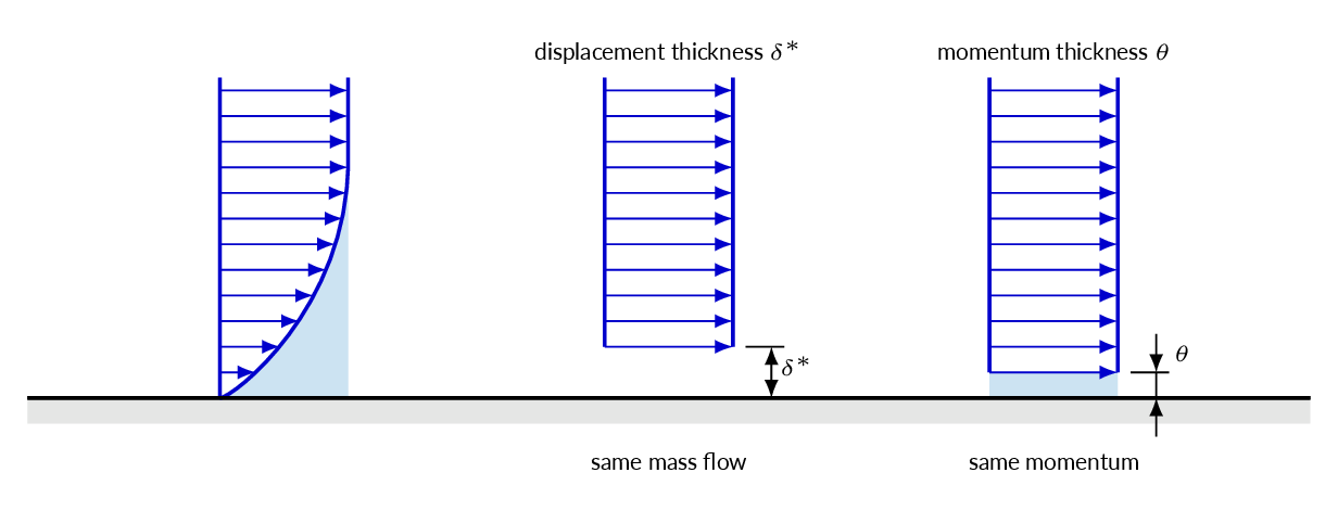
Thus we get an expression for the momentum thickness by integrating the deficit of momentum due to the build up of the velocity profile over the flat plate (\(b\) is the width of the flat plate). It is directly evident that the momentum thickness is related to the Von Kármán integral relation just by comparing the integral expressions.
$$\int_0^\delta \rho u (U-u) bdy=\rho U^2 b \theta\Rightarrow \theta=\int_0^\delta\frac{u}{U}\left(1-\frac{u}{U}\right)dy$$The drag \(D\) for a plate of width \(b\)
$$D(x)=b\int_0^x\tau_w(x)dx\Rightarrow \frac{dD}{dx}=b\tau_w$$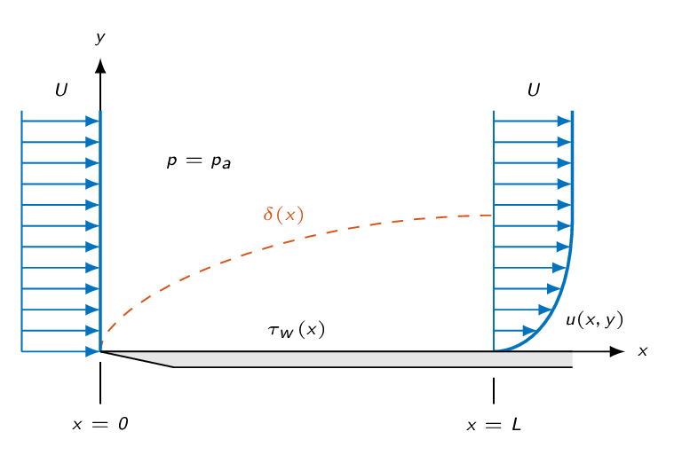
With \(\tau_w\) from the Von Kármán integral relation for a flat plate
$$\frac{\tau_w}{\rho} = \frac{d}{dx}\int_0^\delta u(U-u)dy = \frac{d}{dx}U^2\underbrace{\int_0^\delta \frac{u}{U}(1-\frac{u}{U})dy}_{\theta}=U^2\frac{d\theta}{dx}$$and thus
$$\frac{dD}{dx}=b\rho U^2\frac{d\theta}{dx}\Rightarrow D(x)=\rho bU^2 \theta$$So, the momentum thickness is a measure of the total drag and it is directly related to the Von Kármán integral relation.
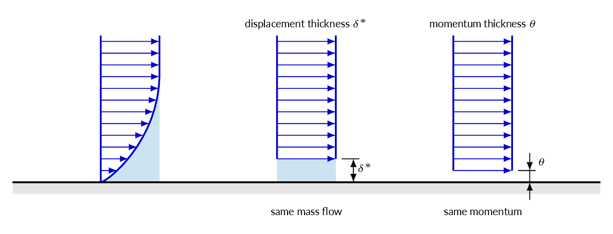
In analogy with the definition of the momentum thickness, the displacement thickness is the distance that a constant-velocity profile must be moved away from the wall to establish a loss in mass flow that represents the deficit of mass flow related to the boundary layer velocity profile. In the same way that we derived a relation for the momentum thickness, the displacement thickness is calculated by integrating the deficit of mass flow through the boundary layer, which gives
$$\int_0^\delta \rho(U-u)bdy=\rho U b\delta^\ast \Rightarrow \delta^\ast = \int_0^\delta \left(1-\frac{u}{U}\right)dy$$The displacement thickness gives an estimate of the displacement of fluid streamlines due to the presence of the boundary layer.
Laminar Flat-Plate Boundary Layer
Parabolic Velocity Profile
Inserting a parabolic velocity profile into the Von Kármán integral relation, we can get estimates of the boundary-layer thickness and the skin friction coefficient (non-dimensional wall-shear stress) that are quite close to the correct values but there is a better alternative, namely the Blasius profile. The parabolic profile assumption is, however, easier to work with.
Blasius Velocity Profile
Blasius approach to solve the boundary-layer equations for laminar flow over a flat plate gives a self-similar solution
$$\dfrac{u}{U}=f(\eta)$$where \(U\) is the freestream velocity and \(\eta\) is a non-dimensional coordinate
$$\eta=y\sqrt{\frac{U}{\nu x}}$$The non-dimensional coordinate corresponds to scale the wall-normal coordinate with the boundary-layer thickness
$$\dfrac{\delta}{x}\propto\dfrac{1}{\sqrt{Re_x}}\Rightarrow\frac{y}{\delta}\propto\frac{y}{x/\sqrt{Re_x}}=\frac{y}{x}\sqrt{\frac{Ux}{\nu}}=y\sqrt{\frac{U}{\nu x}}=\eta$$The Blasius solution is obtained as follows
- Rewrite the boundary layer equations using the stream function
- Rewrite the equation again \(\Psi=f(\eta)\sqrt{\nu Ux}\) where \(\eta\) is the scaled wall-normal coordinate and \(f(\eta)\) is a non-dimensional stream function
- Lots of math ...
The Navier-Stokes equations are reduced to an ordinary differential equation (ODE)
$$f'''+\frac{1}{2}ff''=0$$with the boundary conditions
$$ \left\{ \begin{array}{ll} f(0)=f'(0)=0\\ \\ f'_{\eta\rightarrow\infty}\rightarrow 1.0 \end{array} \right. $$The velocity profile is obtained as
$$\frac{u}{U}=f'(\eta)$$Note! \(u/U\rightarrow 1\) as \(y\rightarrow \infty\) and therefore \(\delta\) is usually defined as the distance from the wall where \(u/U=0.99\)
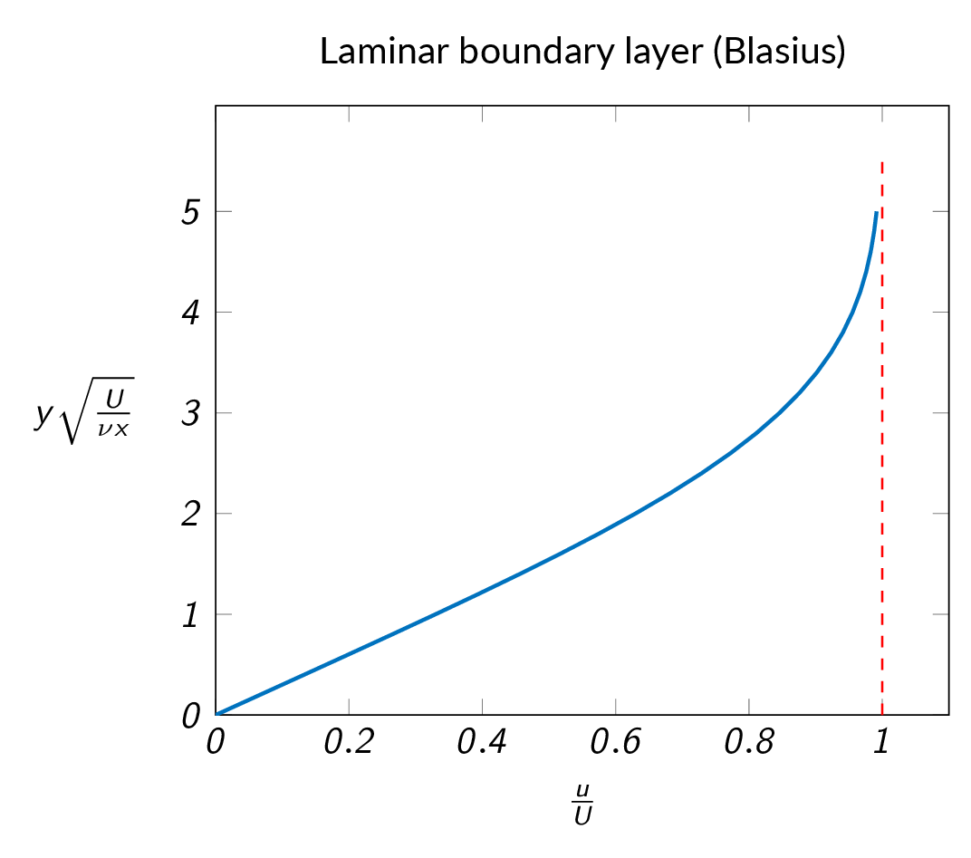
The boundary-layer thickness is obtained from the Blasius solution as follows
$$\delta_{99\%}\sqrt{\frac{U}{\nu x}}\approx 5.0\text{ or }\frac{\delta}{x}\approx \frac{5.0}{\sqrt{Re_x}}$$To get an expression for the wall shear stress, we need the velocity derivative at the wall
$$\tau_w=\mu\left.\frac{\partial u}{\partial y}\right|_{y=0}=\mu U\left[\frac{d}{d\eta}\left(\frac{u}{U}\right)\frac{d\eta}{dy}\right]_{\eta=0}$$ $$\eta=y\sqrt{\dfrac{U}{\nu x}}\Rightarrow\frac{d\eta}{dy}=\sqrt{\frac{U}{\nu x}}\Rightarrow \tau_w=\mu U \sqrt{\frac{U}{\nu x}}\frac{d}{d\eta}\left(\frac{u}{U}\right)_{\eta=0}=\frac{\rho U^2}{\sqrt{Re_x}}\frac{d}{d\eta}\left(\frac{u}{U}\right)_{\eta=0}$$So, we need \(\frac{d}{d\eta}\left(\frac{u}{U}\right)_{\eta=0}\) to calculate the wall-shear stress. The Blasius profile is linear in the near-wall region and it's easy to get the derivative
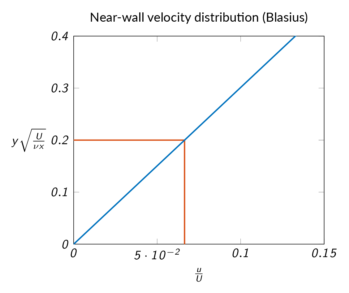
The wall-shear stress is now obtained as
$$\tau_w(x)\approx\frac{0.332\rho^{1/2}\mu^{1/2}U^{3/2}}{x^{1/2}}$$Note! the wall shear stress drops off with increasing distance due to the boundary layer growth.
The fact that the Blasius solution is self-similar means that one single profile describes the velocity distribution for all axial positions in the laminar boundary layer including the boundary layer growth, which is illustrated in the figure below.
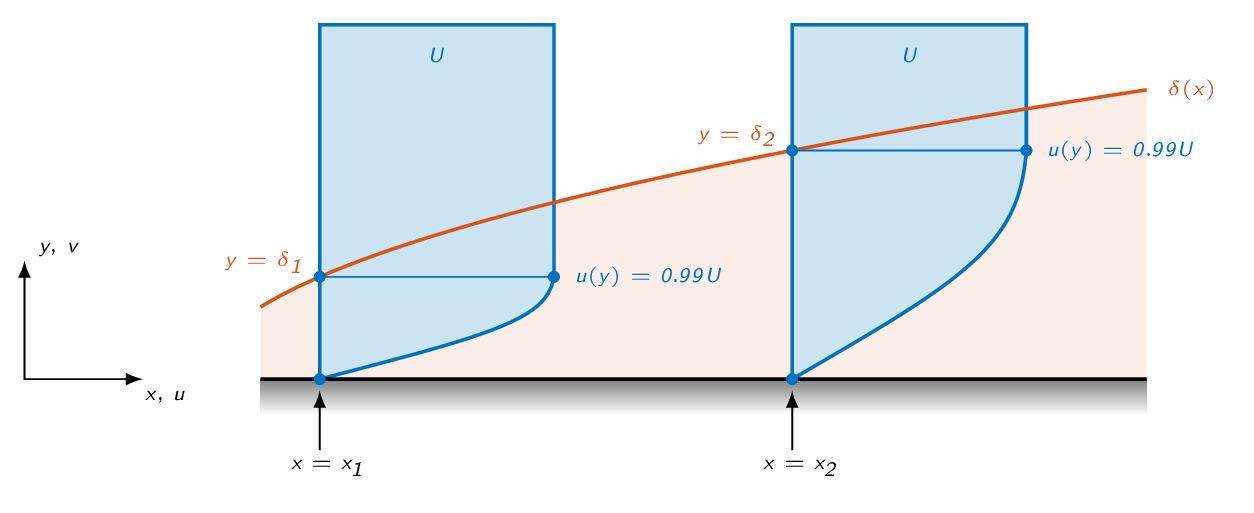 $$\eta(x_1,\delta_1)=\eta(x_2,\delta_2)\Rightarrow\delta_1\sqrt{\dfrac{U}{\nu x_1}}=\delta_2\sqrt{\dfrac{U}{\nu x_2}}$$
$$x_1 < x_2\Rightarrow \sqrt{\dfrac{U}{\nu x_1}} > \sqrt{\dfrac{U}{\nu x_2}}\Rightarrow \delta_1<\delta_2$$
$$\eta(x_1,\delta_1)=\eta(x_2,\delta_2)\Rightarrow\delta_1\sqrt{\dfrac{U}{\nu x_1}}=\delta_2\sqrt{\dfrac{U}{\nu x_2}}$$
$$x_1 < x_2\Rightarrow \sqrt{\dfrac{U}{\nu x_1}} > \sqrt{\dfrac{U}{\nu x_2}}\Rightarrow \delta_1<\delta_2$$
Turbulent Flat-Plate Boundary Layer
For low \(Re_x\), disturbances in the flow are damped out by viscous forces. For somewhat higher Reynolds numbers, friction forces are less important and the flow becomes unstable. For a flat-plate boundary layer, transition occurs at a local Reynolds of about \(Re_x\approx 5.0\times 10^5\). The transition region is short and can be treated as a point (the transition point). The onset of transition from laminar to turbulent is affected by a number of factors such as:
- Turbulence in the freestream
frestream turbulence reduces the critical Reynolds number - Surface roughness
surface roughness does not affect transition significantly if \(Re_\epsilon=\frac{U\epsilon}{\nu}<680\) - Pressure gradient
decreasing pressure in the flow direction has a stabilizing effect on the flow and can delay transition from laminar to turbulent flow
With a smooth surface, no turbulence in the freestream, and zero pressure gradient, the onset of transition can be pushed up to \(Re_x\approx 3.0\times 10^6\). Of course, the critical Reynolds number is not meaningful if the boundary layer is forced to transition.
A turbulent boundary layer grows faster than a laminar boundary layer. The velocity fluctuations \((u^\prime,\ v^\prime,\ w^\prime)\) leads to increased exchange of momentum. Higher turbulence intensity, leads to more effective mixing in the boundary layer. The exchange of momentum means that the velocity close to the wall is higher than for a laminar boundary layer. The high velocity close to the wall and thus high velocity gradients means that the wall shear stress will be higher for a turbulent boundary layer than for a laminar boundary layer.
For the turbulent boundary layer, there is no analytic solution and the velocity profile must be approximated. Prandtl's power law will be used here.
$$\frac{u}{U}\approx\left(\frac{y}{\delta}\right)^{1/7}$$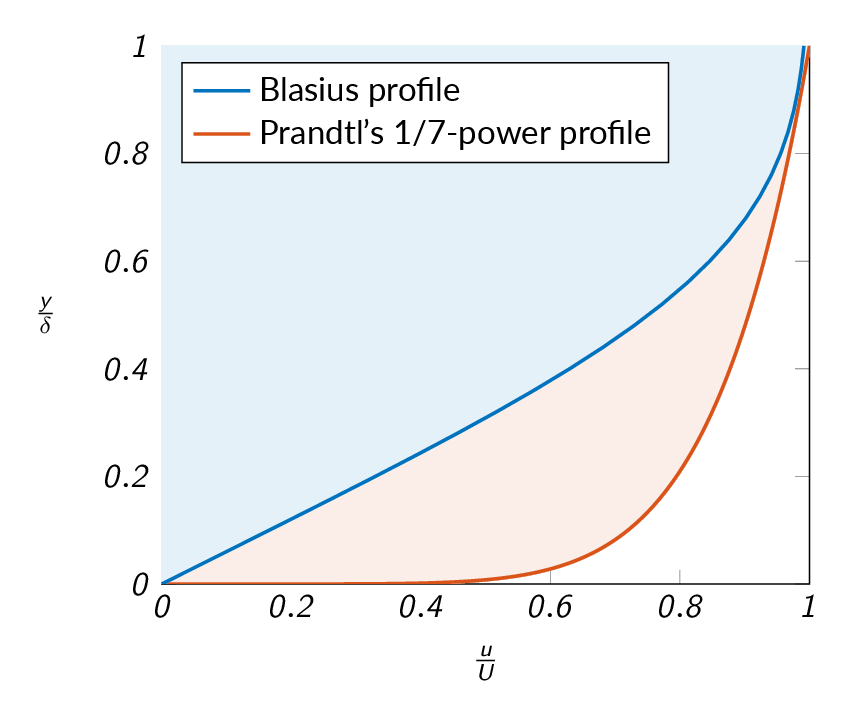
Prandtl suggested the following relation for the skin friction coefficient
$$c_f\approx 0.02 Re_{\delta}^{-1/6}$$The skin friction coefficient can be obtained from the definition of the momentum thickness
$$\tau_w=\rho U^2 \frac{d\theta}{dx}\Rightarrow c_f=2\frac{d\theta}{dx}$$ $$\theta=\int_0^\delta \frac{u}{U}\left(1-\frac{u}{U}\right)dy=\frac{7}{72}\delta$$ $$0.02 Re_{\delta}^{-1/6}=2\frac{d}{dx}\left(\frac{7}{72}\delta\right)$$ $$Re_{\delta}^{-1/6}\approx 9.72 \frac{d\delta}{dx}=9.72 \frac{d (Re_\delta)}{d (Re_x)}$$ $$Re_\delta\approx 0.16 Re_x^{6/7}\text{ or }\frac{\delta}{x}\approx \frac{0.16}{Re_x^{1/7}}$$Note! the turbulent boundary layer grows significantly faster than the laminar \(\delta_{turb}\propto x^{6/7}\) vs \(\delta_{lam}\propto x^{1/2}\)
$$\tau_{w_{turb}}\approx \frac{0.0135 \mu^{1/7} \rho^{6/7} U^{13/7}}{x^{1/7}}$$Friction drops slowly with \(x\), increases nearly as \(\rho\) and \(U^2\), and is rather insensitive to viscosity.
Boundary-Layer Relations
| description | variable | laminar flow (Blasius) | turbulent flow (Prandtl) |
| boundary layer thickness | \(\dfrac{\delta}{x}\) | \(\dfrac{5.0}{\sqrt{Re_x}}\) | \(\dfrac{0.16}{Re_x^{1/7}}\) |
| displacement thickness | \(\dfrac{\delta^\ast}{x}\) | \(\dfrac{1.721}{\sqrt{Re_x}}\) | \(\dfrac{0.02}{Re_x^{1/7}}\) |
| momentum thickness | \(\dfrac{\theta}{x}\) | \(\dfrac{0.664}{\sqrt{Re_x}}\) | \(\dfrac{0.016}{Re_x^{1/7}}\) |
| shape factor | \(H=\dfrac{\delta^\ast}{\theta}\) | 2.59 | 1.29 |
| wall shear stress | \(\tau_w\) | \(0.332\dfrac{\rho U^2}{\sqrt{Re_x}}\) | \(0.0135\dfrac{\rho U^2}{Re_x^{1/7}}\) |
| local skin friction coefficient | \(c_f=\dfrac{2 \tau_w}{\rho U^2}\) | \(\dfrac{0.664}{\sqrt{Re_x}}\) | \(\dfrac{0.027}{Re_x^{1/7}}\) |
| drag coefficient | \(C_D\) | \(\dfrac{1.328}{\sqrt{Re_L}}\) | \(\dfrac{0.031}{Re_L^{1/7}}\) |
The viscous drag for a flat plate boundary layer with transition can be calculated by combining the relations for laminar and turbulent boundary layers. For a long boundary layer the length of the laminar region becomes relatively short in comparison with the length of the turbulent region though.
$$D=b\frac{1}{2}\rho U^2\left[\int_{>0}^{x_{cr}}\frac{0.664}{Re_x^{1/2}}dx + \int_{x_{cr}}^L\frac{0.027}{Re_x^{1/7}}dx\right]$$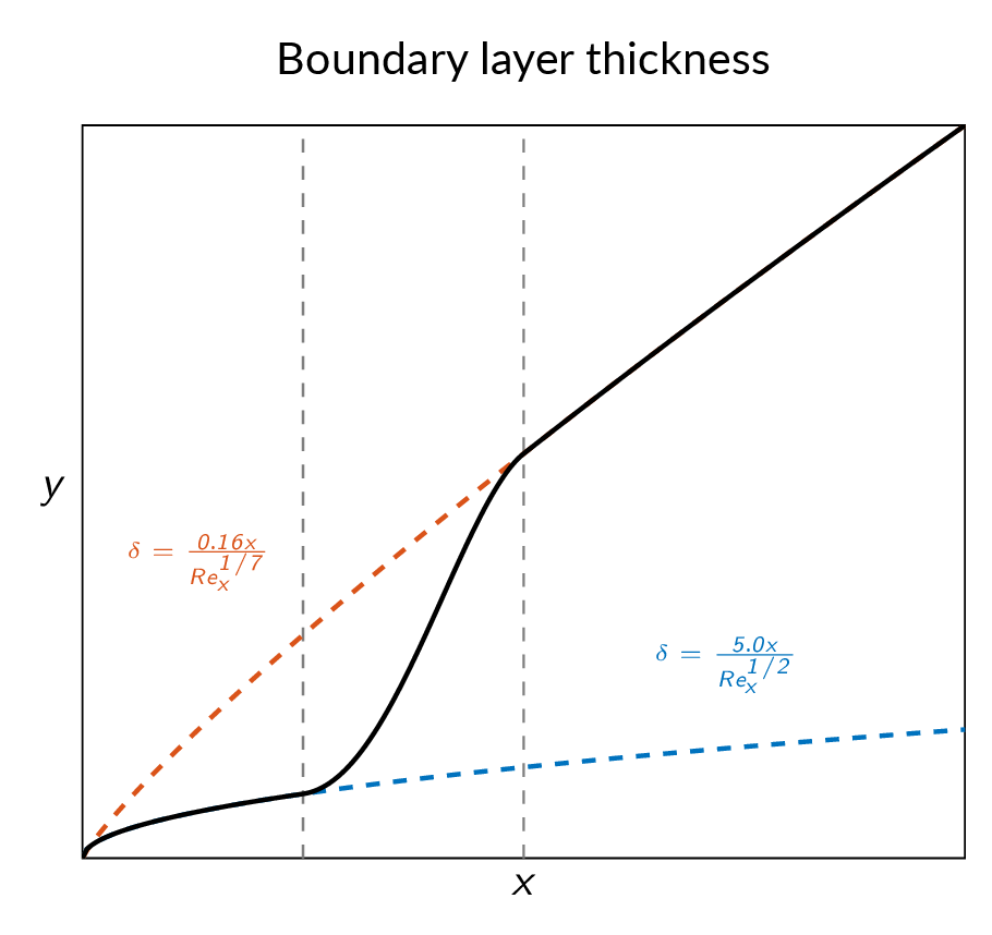
Effects of Surface Roughness
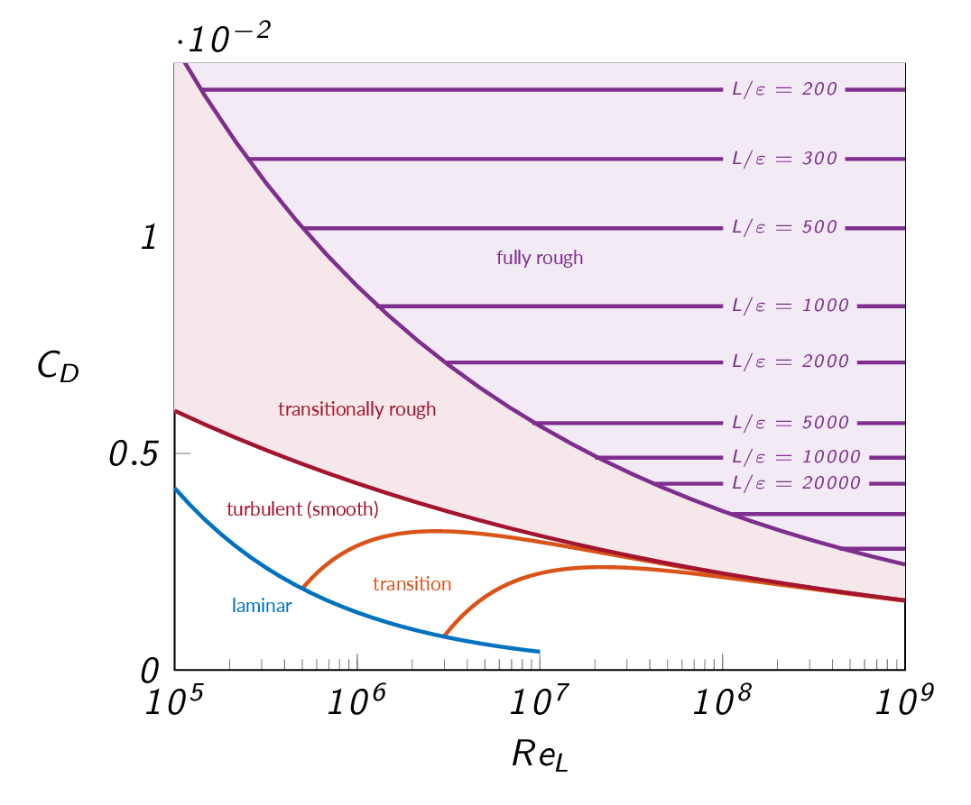
The figure below shows drag coefficient for a flat plate as a function of global Reynolds number for different flow conditions and different surface roughness conditions. As in the case of pipe flows described in chapter 6, surface roughness does not effect laminar flow. Although, in the case of a external boundary layer, surface roughness will effect the onset of transition pushing the critical Reynolds number to lower values. However, for a laminar boundary layer, the drag coefficient (represented by the blue curve in the figure) is given by
$$C_D=\frac{1.328}{Re_L^{1/2}}$$For a turbulent flow over a smooth flat plate, the viscous drag coefficient (represented by the red curve in the figure) is given by
$$C_D=\frac{0.031}{Re_L^{1/7}}$$The drag coefficient for flow with transition are represented by two models, one with a critical Reynolds number of \(5.0\times 10^5\) and one with a critical Reynolds number of \(3.0\times 10^6\)
$$Re_{x,crit}=5.0\times 10^5\Rightarrow C_D=\frac{0.031}{Re_L^{1/7}}-\frac{1440}{Re_L}$$ $$Re_{x,crit}=3.0\times 10^6\Rightarrow C_D=\frac{0.031}{Re_L^{1/7}}-\frac{8700}{Re_L}$$Finally, for turbulent flow over a rough flat plate under fully rough conditions (represented by purple lines in the figure) is given by
$$C_D=(1.89+1.62\log(L/\varepsilon))^{-2.5}$$As you can see from the equation above and the corresponding lines in the figure below, there is no dependence of Reynolds number at fully rough conditions.
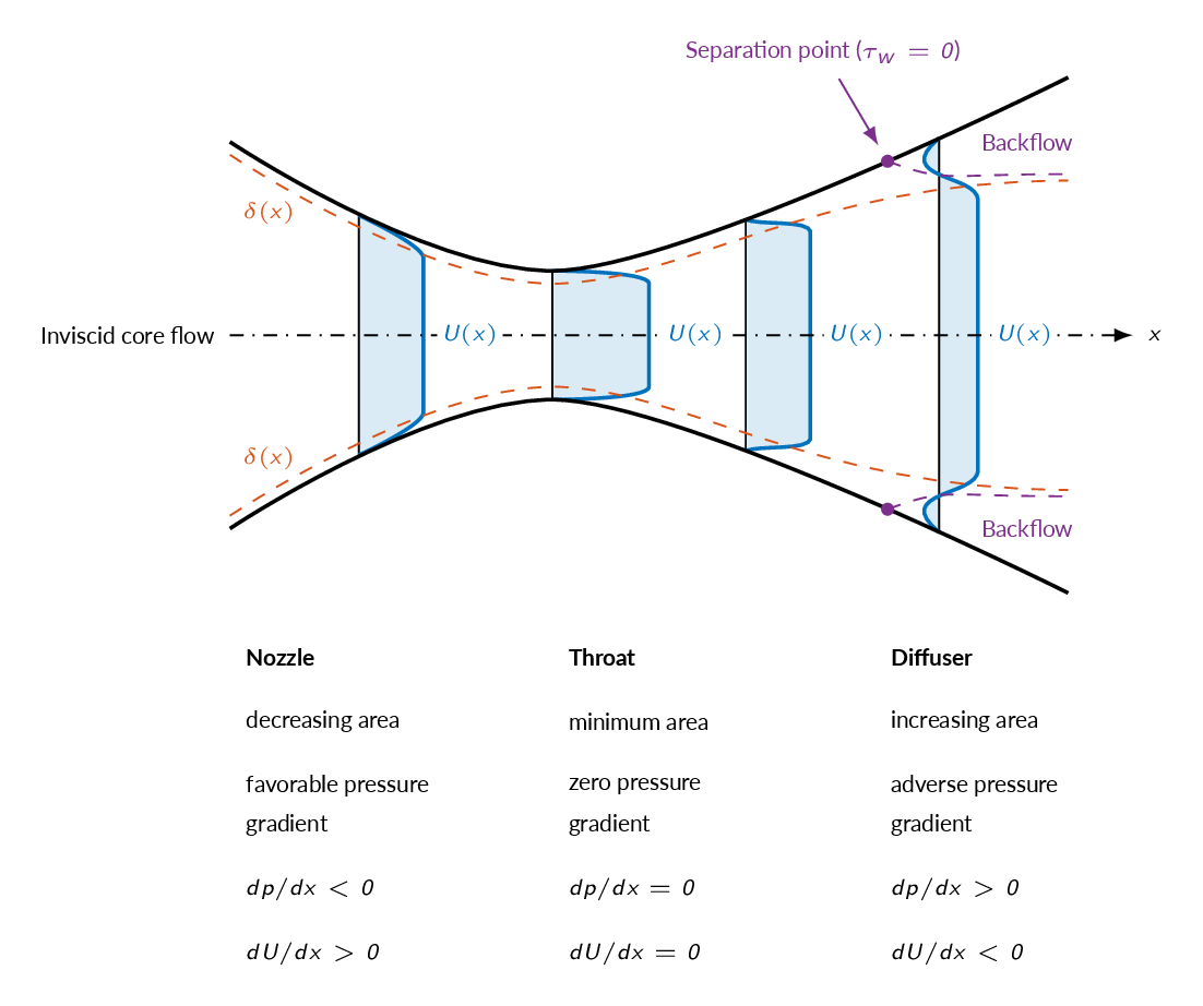
Pressure Gradients and Separation
Pressure Gradient
- Adverse pressure gradient
- pressure increases in the flow direction
- may lead to separation
- Favorable pressure gradient
- pressure decreases in the flow direction
- the flow will not separate
- Separation mechanism
- loss of momentum near the wall
- adverse pressure gradient
- decelerated fluid will force flow to separate from the body
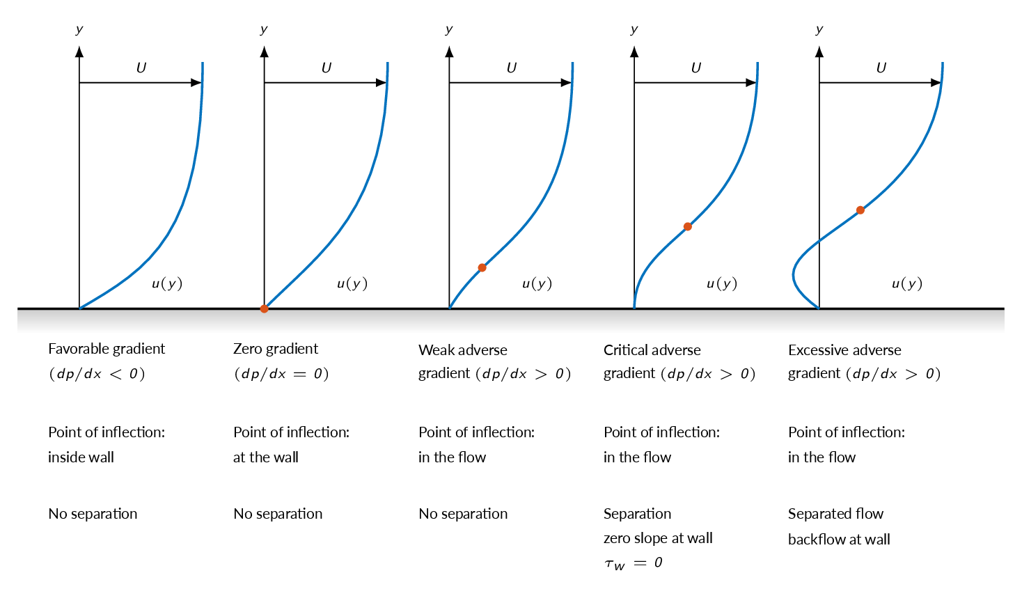
with \(u=v=0\) close at the wall, the boundary layer formulation of the momentum equation reduces to
$$\left.\frac{\partial \tau}{\partial y}\right|_{wall}=\left.\mu \frac{\partial^2 u}{\partial y^2}\right|_{wall}\Rightarrow \left.\frac{\partial^2 u}{\partial y^2}\right|_{wall}= \frac{1}{\mu}\frac{dp}{dx}$$which applies both for laminar and turbulent boundary layers. For adverse pressure gradients \((dp/dx>0)\), \(\partial^2 u/\partial y^2\) will be positive at the wall. At the outer part of the boundary layer the derivative must be negative and thus the derivative will be zero somewhere within the boundary layer. The figure below shows the mechanism behind flow separation.
Forces on Immersed Bodies
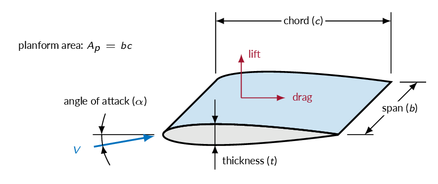
The Force on bodies immersed in flow can be decomposed into two components. The force in the flow direction is called drag force and the component normal to the flow direction is called lift force. Drag and lift are related to the drag coefficient \(C_D\) and the lift coefficient \(C_L\), respectively. The drag and lift coefficients are defined as follows
$$C_D=\dfrac{2 F_D}{\rho V^2 A}$$ $$C_L=\dfrac{2 F_L}{\rho V^2 A}$$The forces are normalized by dynamics pressure and a characteristic area. The definition of the characteristic area depends body shape. For a blunt body like a cylinder, sphere, or a car it is the projected area in the direction of the flow. For a thin object like a flat plate or a wing, the characteristic area is the plan-form area, i.e. the projected area in the direction normal to the flow (for the wing this means the area that you see if looking at the wing from above).
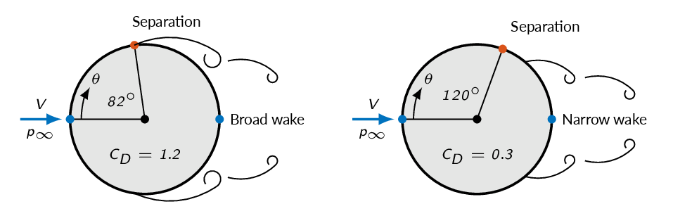
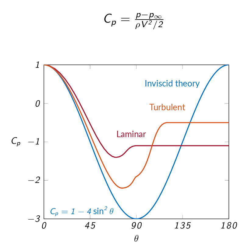
For a body immersed in flow that, unlike the flat plate, has a thickness, there are two contributions to the total drag force. The drag force is the sum of the viscous/friction the force appearing due to the pressure difference over the body. The figures below shows schematic representations of the flow around a cylinder. For the cylinder to the left, a laminar boundary layer is built up over the cylinder surface while the boundary layer on the cylinder to the right is turbulent. Since the turbulent boundary layer leads to higher velocity and thus higher momentum close to the wall (compare the laminar (Blasius) and turbulent (Prandtl) velocity profiles above), the turbulent boundary layer will be less prone to separate from the cylinder surface. Therefore, the separation point is further back on the cylinder in the turbulent case and thus the width of the wake on the backside of the cylinder is smaller than for the laminar case. Postponing the separation is beneficial for pressure recovery as can be seen in the graph below. A smaller low-pressure region means that the pressure force on the cylinder will be smaller in the turbulent case and thus the pressure drag is smaller. However, since the velocity close to the wall is higher in the turbulent case, the velocity gradient at the wall is higher, which in turn means that the viscous drag will be higher in the turbulent case.
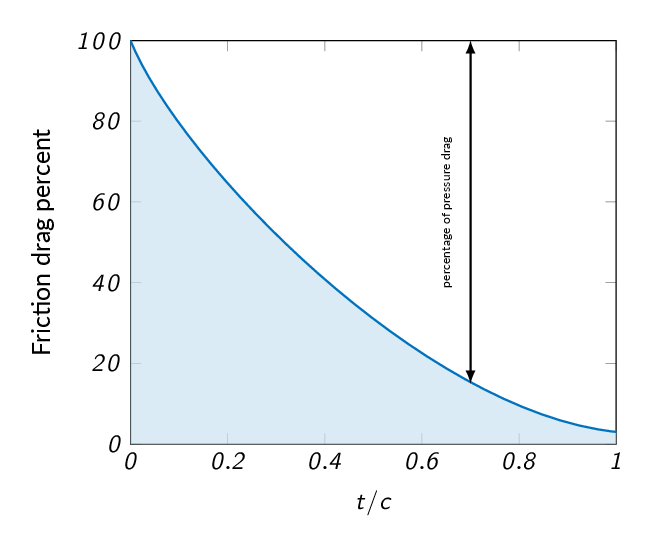
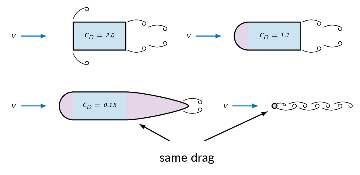
The relative importance of pressure drag and friction drag depends on the shape of the body as illustrated below.

There are several ways by which separation can be avoided or postponed (see examples listed below).
- Decrease magnitude of adverse pressure gradient
- Guide vanes
- Streamlining (see example below)
- Remove decelerated fluid
- Boundary layer suction
- Increase near-wall momentum
- Injection of high-velocity fluid in the near-wall region
- Force transition to turbulence
- surface roughness
- surface irregularities (dimples on the surface of a golf ball)
- trip wires
The figure below shows schematically how streamlining of a body can be used to decrease pressure drag. It should be noted, however, that the decrease in pressure drag comes with a penalty in the form of increased friction drag since the area that is in contact with the fluid (the wetted area) is increased significantly.
Study Guide
The questions below are intended as a "study guide" and may be helpful when reading the text book.
- Make a schematic sketch of the velocity profile in a flat-plate boundary layer showing the extent of the viscous region at \(Re_L=10\) and \(Re_L=10^7\), respectively. How does the extent of the viscous region \(\delta\) relate to the characteristic length, \(L\), for the two Reynolds numbers? Indicate what parts of the boundary layer that is laminar and turbulent respectively as well as the transition region.
- Make a schematic sketch of the flow over a cylinder at \(Re_D=10^5\). Indicate the stagnation point, separation points and the wake region.
- The boundary layer equations are derived from the continuity equation and the Navier-Stokes equation on non-dimensional form (MTF053 Equation-for-Boundary-Layer-Flows.pdf)
- Define the non-dimensional properties \(x^\ast\), \(u^\ast\), and \(p^\ast\) and explain the included properties.
- Give the order of magnitude of \(x^\ast\), \(u^\ast\), and \(p^\ast\) that holds for larger part of the boundary layer. The estimation of magnitude is made using the following terms \(\partial u^\ast/\partial x^\ast\), \(\partial u^\ast/\partial y^\ast\), \(\partial^2 u^\ast/\partial x^{\ast^2}\), and \(\nu^\ast\). Use relevant figures to justify the estimation of the derivatives.
- What assumption is made to be able to derive the boundary layer equations?
- Show that the static pressure is independent of the distance from the wall in a laminar two-dimensional boundary layer. Use the non-dimensional form of the \(y\)-component of the Navier-Stokes equations
$$u^\ast\dfrac{\partial v^\ast}{\partial x^\ast}+v^\ast\dfrac{\partial v^\ast}{\partial y^\ast}=-\dfrac{\partial p^\ast}{\partial y^\ast}+\dfrac{1}{Re}\left(\dfrac{\partial^2 v^\ast}{\partial x^{\ast^2}}+\dfrac{\partial^2 v^\ast}{\partial y^{\ast^2}}\right)$$
The following size estimates can be assumed to hold (does not need to be proved): \(u^\ast\sim 1\), \(v^\ast\sim\delta^\ast\), and \(Re\sim\delta^{\ast^{-2}}\)
note: here \(\delta^\ast\) is the non-dimensional boundary layer thickness, not the displacement thickness - How does the laminar and turbulent boundary layer equations differ? How does this effect the possibility to solve the equations?
- Show using the Bernoulli equation (with small differences in elevation) that the pressure gradient for the flow over a flat plate depends on the density, the derivative of the freestream velocity, and the freestream velocity. Justify the use of the Bernoulli equation for this purpose.
- Describe in words the steps taken in Blasius solution of the boundary layer equations for laminar flow over a flat plate.
- For laminar flow over a flat plate, the velocity profile is self-similar - what does that mean?
- For a laminar boundary layer over a flat plate, the local wall shear stress coefficient \(c_f\) can be obtained as $$c_f=\dfrac{0.664}{\sqrt{Re_x}}$$ The wall shear stress coefficient, \(c_f\), is related to the wall shear stress, \(\tau_w\), and the free stream velocity, \(U\), as $$c_f=\dfrac{2 \tau_w}{\rho U^2}$$ Show how to obtain the total friction force (the flat plate drag), \(D\), for one side of a flat plate with the length \(L\). Derive an expression for the drag force on non-dimensional form using the drag coefficient \(C_D\).
- Name two alternative ways to measure the boundary layer thickness than \(\delta\). How can these measures be interpreted physically?
- Derive von Kármán's momentum integral relation $$\tau_w=\rho U^2\dfrac{d\theta}{dx}$$ starting from $$D(x)=\rho bU^2\theta$$ where $$\theta=\int_0^\delta\dfrac{u}{U}\left(1-\dfrac{u}{U}\right)dy$$ Describe how to derive an approximate solution for the boundary layer thickness and the wall shear stress for laminar flow over a flat plate using the von Kármán momentum integral relation.
- In what way is the transition location effected by (assume other properties to be constant)
- increased freestream velocity \(U\) for a given \(Re_{x,tr}\)
- surface roughness \(\varepsilon\)
- freestream turbulence
- positive pressure gradient
- Show how the velocity profile as well as its first and second derivative and the pressure gradient change in a boundary layer when the flow separates
- The drag coefficient, \(C_D\), for cylinder flow is drastically changed as the boundary layer becomes turbulent (before separating). Show schematically how \(C_D\) varies with the Reynolds number, \(Re_D\), and indicate the location transition to turbulence and separation.
- The drag coefficient, \(C_D\), can be divided into two components, which two components? What phenomena are associated with each of the two components?
- Make a schematic representation of the pressure distribution around a cylinder for inviscid flow (potential flow), viscous flow with laminar and turbulent separation respectively. Explain why the pressure varies the way it does. Which of the three cases will give the lowest and highest pressure drag?
- Why do dimpled golf balls have lower pressure drag than golf balls with smooth surfaces?
| Document Archive | ||
| MTF053_C07.pdf | lecture notes chapter 7 | |
| MTF053_Equations-for-Boundary-Layer-Flows.pdf | Complementary material - Derivation of simplified flow equations for boundary layer flows | |
| MTF053_Turbulence.pdf | Complementary material - Turbulent flow theory | |
| MTF053_Formulas-Tables-and-Graphs.pdf | A collection of formulas, tables, and graphs | |
| MTF053_Study-Guide.pdf | A collection of theory questions that give a good representation of the theory covered in the course | |