Chapter 6
Viscous Flow in Ducts
Viscous Flow in Ducts
Overview
In chapter 6, the theory derived in previous sections is applied to the application viscous flows in ducts. As a part of the derivation of relations for estimation of viscous losses in pipe flows, turbulence theory is introduced in this chapter. Turbulence is of course not specific for the pipe flow application, it appears in all types of flows, but in this book it is nevertheless introduced in this context. Other important concepts introduced in this chapter are; transition to turbulence and critical Reynolds number, the Darcy friction factor, Reynolds decomposition, boundary layers, surface roughness, and, last but not least, the Reynolds-Averaged Navier-Stokes (RANS) equations.
Roadmap
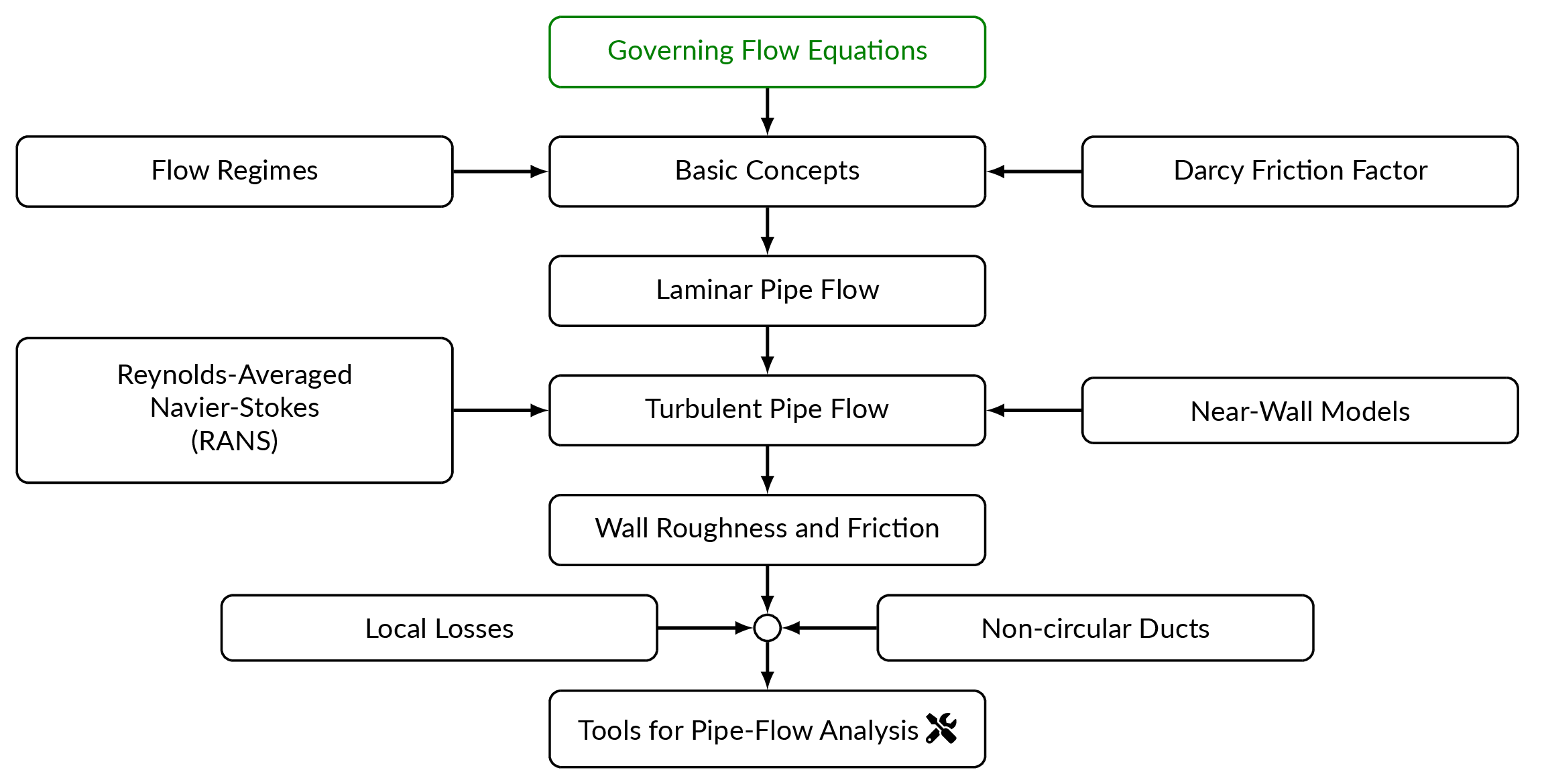
Flow Regimes
The character of pipe flows, and flows in general, are to a high degree defined by the Reynolds number. As you might remember from chapter 5, the Reynolds number describes the relation between inertial forces and viscous forces. A low Reynolds number means that the flow is dominated by viscosity. Transition to turbulence will occur in a range of Reynolds numbers that is specific for the application and for pipe flows an excepted value is \(Re_{D_{critical}}=2300\). With careful design (smooth surfaces and low turbulence intensity in the incoming flow), the onset of transition can be pushed to higher values but \(Re_{D_{critical}}=2300\) can be used as a rule of thumb. In a laminar flow at low Reynolds number, small instabilities will be killed by viscosity. Increasing the Reynolds number small bursts of turbulence can be observed in the flow but will die out due to viscous effects. When the critical Reynolds number is approached, the bursts of turbulence in the laminar flow will be more frequent and eventually, the flow will be turbulent. The fluctuations in a turbulent flow are random and there's a continuous spectrum of frequencies. Velocity fluctuations are typically 1-20 percent of the average velocity. The fluctuations leads to increased mixing in the flow and that in turn leads to higher velocities in the near-wall regions.
The great majority of our analyses are concerned with laminar flow or with turbulent flow, and one should not normally design a flow operation in the transition region.
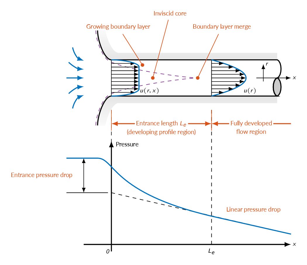
At the wall the flow velocity must be zero (no-slip condition) and a boundary layer will be formed where the velocity increases gradually from zero velocity at the wall. Pipe/duct flows are confined, which means the the growth of boundary layers are limited by the size of the pipe cross section and the boundary layers will meet at the center of the pipe (see figure above). When the flow enters the pipe, only a thin region close to the wall will be effected by viscosity. Outside of the thin boundary layer the flow will be inviscid. Moving downstream the pipe, the inviscid core decreases in size as the boundary layer grows and eventually the boundary layer meets at the center of the pipe and the flow is fully developed.
The Darcy Friction Factor
The Darcy friction factor \(f\) is a function of Reynolds number (\(Re_D\)), the wall roughness (\(\varepsilon/D\)), and duct shape and is defined as
$$h_f=f_D\frac{L}{d}\frac{V^2}{2g}$$where \(h_f\) is the head loss.
We will get the head loss by analyzing a pipe like the one depicted below using the steady-flow energy equation between two stations in the pipe.
$$\left(\frac{p}{\rho g}+\alpha\frac{V^2}{2g}+z\right)_1=\left(\frac{p}{\rho g}+\alpha\frac{V^2}{2g}+z\right)_2+h_f$$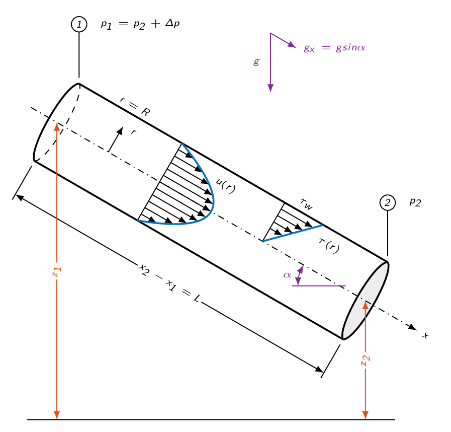
The flow is fully developed, which means that the average velocity is constant (\(V_1=V_2\)) and the velocity profile has the same shape at both stations (\(\alpha_1=\alpha_2\)), which means that the equation above may be rewritten as
$$h_f=(z_1-z_2)+\left(\frac{p_1-p_2}{\rho g}\right)=\Delta z + \frac{\Delta p}{\rho g}$$Next step is to evaluate the momentum equation between stations 1 and 2.
$$\sum F_x=\Delta p(\pi R^2)+\rho g (\pi R^2)L\sin\alpha - \tau_w(2\pi R)L=\dot{m}(V_2-V_1)=0$$and thus
$$\frac{\Delta p}{\rho g}+\Delta z=\frac{4\tau_w}{\rho g}\frac{L}{d}$$Going back to the energy equation, we see that the left-hand-side of the equation above is equal to the head loss \(h_f\).
$$h_f=\frac{4\tau_w}{\rho g}\frac{L}{d}$$Inserting the head loss as defined above into the expression defining the Darcy friction factor gives.
$$f_D=\frac{8\tau_w}{\rho V^2}$$Fully-Developed Laminar Pipe Flow
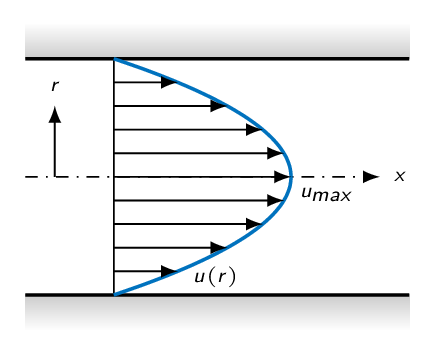
For fully-developed laminar flow in a circular pipe with the diameter \(D\), the velocity profile is given by
$$u(r)=u_{max}\left(1-\left(\frac{r}{R}\right)^2\right)$$and thus
$$\tau_w= \mu \left|\frac{du}{dr}\right|_{r=R}=\frac{4\mu V}{R}=\frac{8\mu V}{D}$$ $$f_D=\frac{8\tau_w}{\rho V^2}=\{\tau_w=\frac{8\mu V}{D}\}=\frac{64 \mu}{\rho V D}=\frac{64}{Re_D}$$Note! in laminar flow, the friction factor is inversely proportional to the Reynolds number.
Reynolds-Averaged Navier-Stokes (RANS)
The figure below gives a schematic representation of a velocity signal (left) and a pressure signal (right) measured by a probe placed at a fixed position in a turbulent flow. The unsteady turbulent flow is impossible to analyze analytically (and, unless tremendous computational resources are used, also numerically). Fortunately, quite often the time-averaged flow is of greater interest than the unsteady flow. Reynolds proposed a method to get a set equations describing the time-averaged flow field - the Reynolds-Averaged Navier-Stokes (RANS) equations.
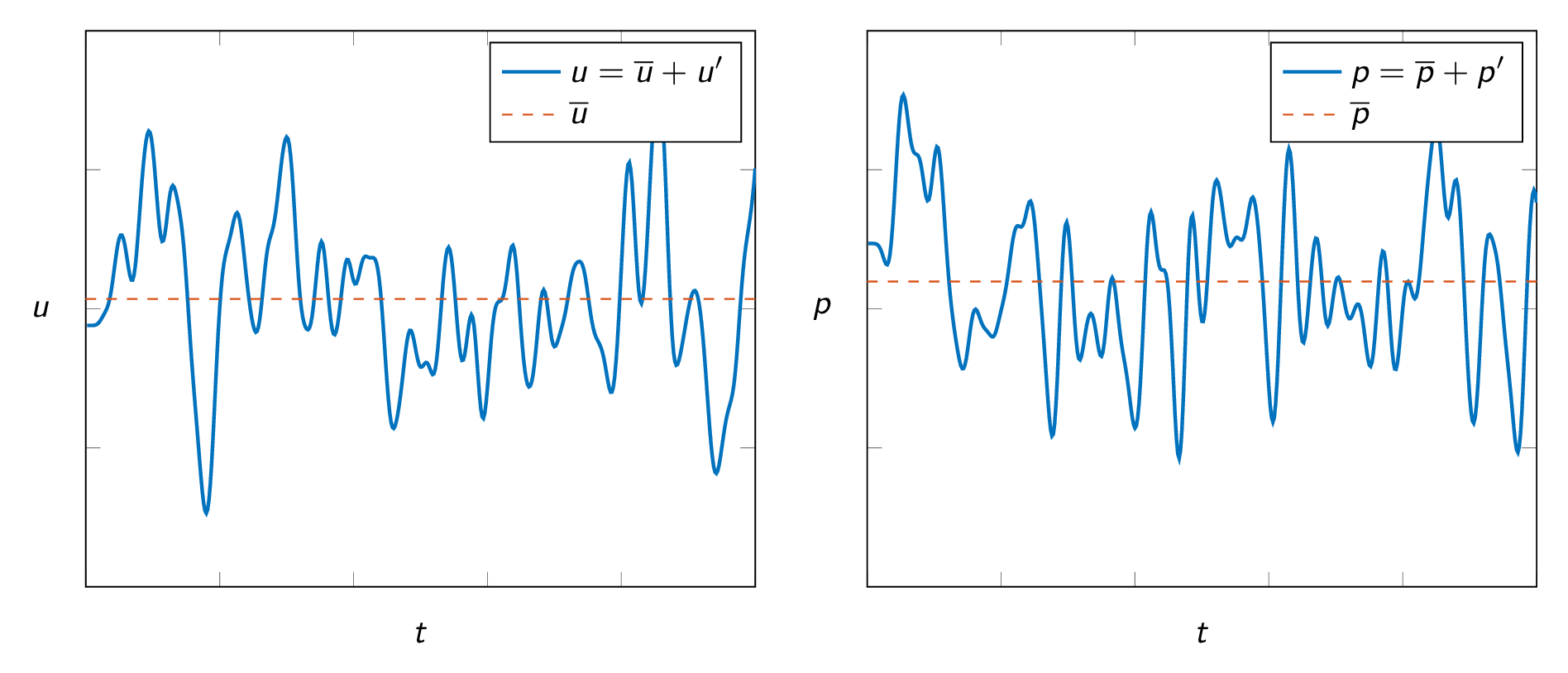
In the figures above, quantities with a bar above are time-averages and primed quantities denotes the fluctuations around the mean value. Reynolds decomposition implies that flow quantities are decomposed into an average and a fluctuation. The time average of the \(x\)-component of the velocity is obtained as
$$\overline{u}=\frac{1}{T}\int_0^Tudt$$The corresponding velocity fluctuation is obtained as
$$u^\prime = u - \overline{u}$$and thus we can see that the time average of the fluctuation is zero.
$$\overline{u^{\prime}}=\frac{1}{T}\int_0^T(u-\overline{u})dt=\overline{u}-\overline{u}=0$$The mean square of the fluctuations are, however, not zero.
$$\overline{u^{\prime 2}}=\frac{1}{T}\int_0^Tu^{\prime 2} dt \ne 0$$Reynolds' idea was to split all properties into mean and fluctuating parts:
$$u=\overline{u}+u^\prime,\ v=\overline{v}+v^\prime,\ w=\overline{w}+w^\prime,\ p=\overline{p}+p^\prime$$Then insert the decomposed variables into the governing equations and time average the equations.
Continuity:
$$\frac{\partial u}{\partial x}+\frac{\partial v}{\partial y}+\frac{\partial w}{\partial z}=0$$inserting the decomposed variables
$$\frac{\partial \overline{u}}{\partial x}+\frac{\partial \overline{v}}{\partial y}+\frac{\partial \overline{w}}{\partial z}+\frac{\partial u^{\prime}}{\partial x}+\frac{\partial v^{\prime}}{\partial y}+\frac{\partial w^{\prime}}{\partial z}=0$$time averaging the equation gives
$$\frac{\partial \overline{u}}{\partial x}+\frac{\partial \overline{v}}{\partial y}+\frac{\partial \overline{w}}{\partial z}=0$$and thus as a consequence
$$\frac{\partial u^{\prime}}{\partial x}+\frac{\partial v^{\prime}}{\partial y}+\frac{\partial w^{\prime}}{\partial z}=0$$Momentum (\(x\)-direction):
$$\rho\left(\frac{\partial u}{\partial t}+u\frac{\partial u}{\partial x}+v\frac{\partial u}{\partial y}+w\frac{\partial u}{\partial z}\right)=-\frac{\partial p}{\partial x}+\rho g_x+\mu\left(\frac{\partial^2 u}{\partial x^2}+\frac{\partial^2 u}{\partial y^2}+\frac{\partial^2 u}{\partial z^2}\right)$$inserting the decomposed variables
$$ \begin{array}{ll} \rho\left( \dfrac{\partial \overline{u}}{\partial t}+ \dfrac{\partial u^{\prime}}{\partial t}\right)+\\ \\[-10pt] \rho\left( \overline{u}\dfrac{\partial \overline{u}}{\partial x}+ \overline{u}\dfrac{\partial u^{\prime}}{\partial x}+ u^{\prime}\dfrac{\partial \overline{u}}{\partial x}+ u^{\prime}\dfrac{\partial u^{\prime}}{\partial x}\right)+\\ \\[-10pt] \rho\left( \overline{v}\dfrac{\partial \overline{u}}{\partial y}+ \overline{v}\dfrac{\partial u^{\prime}}{\partial y}+ v^{\prime}\dfrac{\partial \overline{u}}{\partial y}+ v^{\prime}\dfrac{\partial u^{\prime}}{\partial y}\right)+\\ \\[-10pt] \rho\left( \overline{w}\dfrac{\partial \overline{u}}{\partial z}+ \overline{w}\dfrac{\partial u^{\prime}}{\partial z}+ w^{\prime}\dfrac{\partial \overline{u}}{\partial z}+ w^{\prime}\dfrac{\partial u^{\prime}}{\partial z} \right)=\\ \\[-10pt] -\dfrac{\partial \overline{p}}{\partial x}-\dfrac{\partial p^{\prime}}{\partial x}+\rho g_x+ \mu\left(\dfrac{\partial^2 \overline{u}}{\partial x^2}+\dfrac{\partial^2 \overline{u}}{\partial y^2}+\dfrac{\partial^2 \overline{u}}{\partial z^2}+ \dfrac{\partial^2 u^{\prime}}{\partial x^2}+\dfrac{\partial^2 u^{\prime}}{\partial y^2}+\dfrac{\partial^2 u^{\prime}}{\partial z^2}\right) \end{array} $$time averaging the equation gives
$$ \begin{array}{ll} \rho\left( \dfrac{\partial \overline{u}}{\partial t}+ \overline{u}\dfrac{\partial \overline{u}}{\partial x}+ \overline{v}\dfrac{\partial \overline{u}}{\partial y}+ \overline{w}\dfrac{\partial \overline{u}}{\partial z}+ \overline{u^{\prime}\dfrac{\partial u^{\prime}}{\partial x}}+ \overline{v^{\prime}\dfrac{\partial u^{\prime}}{\partial y}}+ \overline{w^{\prime}\dfrac{\partial u^{\prime}}{\partial z}} \right)=\\ \\[-10pt] -\dfrac{\partial \overline{p}}{\partial x}+\rho g_x+ \mu\left(\dfrac{\partial^2 \overline{u}}{\partial x^2}+\dfrac{\partial^2 \overline{u}}{\partial y^2}+\dfrac{\partial^2 \overline{u}}{\partial z^2}\right) \end{array} $$The fluctuation products on the left-hand-side are rewritten as
$$ \overline{u^{\prime}\dfrac{\partial u^{\prime}}{\partial x}}+ \overline{v^{\prime}\dfrac{\partial u^{\prime}}{\partial y}}+ \overline{w^{\prime}\dfrac{\partial u^{\prime}}{\partial z}} = \dfrac{\partial \overline{u^{\prime}u^{\prime}}}{\partial x}+\dfrac{\partial \overline{u^{\prime}v^{\prime}}}{\partial y}+\dfrac{\partial \overline{u^{\prime}w^{\prime}}}{\partial z}- \overline{u^{\prime}\underbrace{\left(\dfrac{\partial u^{\prime}}{\partial x}+\dfrac{\partial v^{\prime}}{\partial y}+\dfrac{\partial w^{\prime}}{\partial z}\right)}_{=0}} $$and thus
$$\begin{array}{ll} &\rho\dfrac{D \overline{u}}{Dt}=-\dfrac{\partial \overline{p}}{\partial x}+\rho g_x+\dfrac{\partial }{\partial x}\left(\mu\dfrac{\partial \overline{u}}{\partial x}-\rho \overline{u^{\prime 2}}\right)+\\ &\\ &\dfrac{\partial }{\partial y}\left(\mu\dfrac{\partial \overline{u}}{\partial y}-\rho \overline{u^{\prime}v^{\prime}}\right)+\dfrac{\partial }{\partial z}\left(\mu\dfrac{\partial \overline{u}}{\partial z}-\rho \overline{u^{\prime}w^{\prime}}\right) \end{array}$$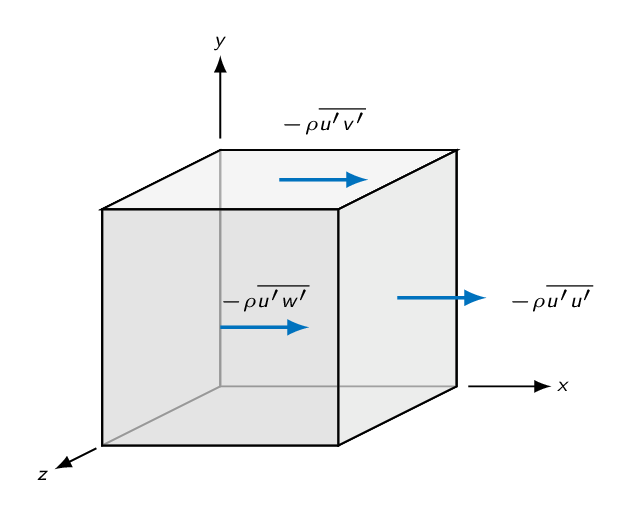
By applying Reynolds' decomposition to our governing equations, we have introduced a number of new unknowns. The number of equations is the same as before. This is often referred to as the closure problem of turbulence. The three correlation terms \(-\rho \overline{u^{\prime 2}}\), \(-\rho \overline{u^{\prime}v^{\prime}}\), and \(-\rho \overline{u^{\prime}w^{\prime}}\) are called Reynolds stresses or turbulent stresses. In duct and boundary layer flow, the stress \(-\rho \overline{u^{\prime}v^{\prime}}\), associated with the direction normal to the wall, is dominant and the others are often neglected.
$$\rho\frac{D \overline{u}}{Dt}\approx-\frac{\partial \overline{p}}{\partial x}+\rho g_x+\frac{\partial \tau}{\partial y}$$where
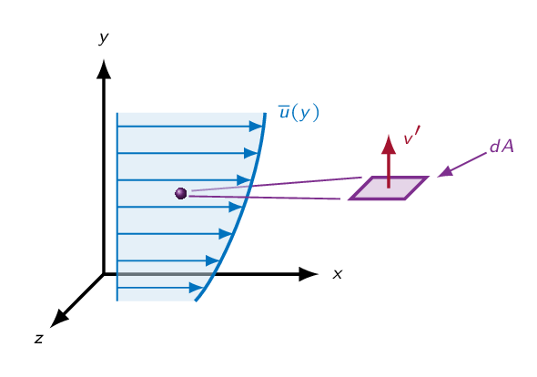
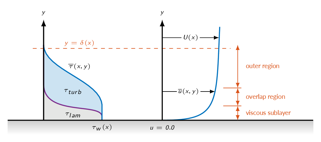
$$\tau=\mu\frac{\partial \overline{u}}{\partial y}-\rho \overline{u^{\prime}v^{\prime}}=\tau_{lam}+\tau_{turb}$$Imagine an infinitesimal surface in a boundary layer as depicted in the figure below. The mass flow through surface element will be
$$\dot{m}_y=\rho v^\prime dA$$.A momentum balance in \(x\)-direction gives
$$F_x=\dot{m}_y u=\rho v^\prime \left(\overline{u}+u^\prime\right) dA$$ $$\tau_{dA}=-\frac{\overline{F}_x}{dA}=-\overline{\rho v^\prime \left(\overline{u}+u^\prime\right)}=-\rho\overline{v^\prime \overline{u}}-\rho\overline{u^\prime v^\prime}=\left\{\overline{v^\prime\overline{u}}=\overline{v^\prime}\overline{u}=0\right\}=-\rho\overline{u^\prime v^\prime}$$Thus, \(-\rho\overline{u^\prime v^\prime}\) can be interpreted as a shear stress.
Introducing turbulent viscosity \(\mu_t\) defined such that
$$-\rho \overline{u^{\prime}v^{\prime}}=\mu_t\frac{\partial \overline{u}}{\partial y}$$This is Boussinesq's assumption and leads to the following expression for the shear stress \(\tau\)
$$\tau=\mu\frac{\partial \overline{u}}{\partial y}-\rho \overline{u^{\prime}v^{\prime}}=(\mu+\mu_t)\frac{\partial \overline{u}}{\partial y}$$Close to the wall, the shear stress is dominated by molecular viscosity while further out from the wall in a turbulent boundary layer, the turbulent stress will dominate over the laminar shear stress.
Near-wall Modeling Concepts
For boundary layer flows, the momentum equation reduces to
$$\rho\left(\overline{u}\dfrac{\partial \overline{u}}{dx}+\overline{v}\dfrac{\partial \overline{u}}{dy}\right)=-\dfrac{d \overline{p}}{dx}+\rho g_x+(\mu+\mu_t)\dfrac{\partial \overline{u}}{\partial y}$$Close to the wall, the velocity is approaching zero and therefore the left-hand side of the equation above is zero.
$$\dfrac{\partial \tau}{\partial y}=\dfrac{d \overline{p}}{dx}-\rho g_x$$ $$\tau(y)=\left(\frac{d \overline{p}}{dx}-\rho g_x\right)y+C$$ $$\tau(0)=C=\tau_w \Rightarrow \tau(y)=\left(\frac{d \overline{p}}{dx}-\rho g_x\right)y+\tau_w$$At the wall, the shear stress is equal to the wall-shear stress
$$y\rightarrow 0 \Rightarrow \tau(y)\rightarrow \tau_w$$In fact, assuming that the shear stress (\(\tau\)) is constant and equal to the wall-shear stress (\(\tau_w\)) is a valid assumption in the near-wall region (some distance from the wall but still close) as long as the pressure gradient is moderate. Outside of the near-wall region, inertial effects has to be accounted for, i.e., \(D\overline{u}/Dt\) will not be zero and thus the shear stress will not be equal to the wall-shear stress.
A turbulent boundary layer may be divided into different regions where the physical processes leading to shear stress are clearly distinguishable.
- The viscous sublayer
- the shear stress is dominated by molecular viscosity (\(\mu\))
- The buffer region
- molecular viscosity (\(\mu\)) and turbulent viscosity (\(\mu_t\)) are equally important
- The log layer
- the shear stress is dominated by turbulent viscosity (\(\mu_t\))
- The outer region
- inertial effects must be accounted for
The Viscous Sublayer
Close to the wall, in the viscous sublayer, the velocity fluctuations will approach zero and thus the shear stress is dominated by molecular viscosity (\(\mu\)).
$$\tau=\mu\frac{\partial \overline{u}}{\partial y}$$ $$\tau=\mu\frac{\partial \overline{u}}{\partial y} \Rightarrow \overline{u}(y)=\frac{\tau_w}{\mu}y+C$$ $$\overline{u}(0)=0\Rightarrow C=0\Rightarrow\overline{u}(y)=\frac{\tau_w}{\mu}y$$Introducing friction velocity defined as
$$u^{\ast}=\sqrt{\frac{\tau_w}{\rho}}$$and thus
$$\overline{u}(y)=\frac{\tau_w}{\mu}y=\frac{\rho {u^{\ast}}^2 y}{\mu}=\frac{ {u^{\ast}}^2 y}{\nu}$$which can be rewritten as:
$$\underbrace{\frac{\overline{u}}{u^{\ast}}}_{u^+}=\underbrace{\frac{u^{\ast} y}{\nu}}_{y^+}$$The viscous sublayer model is valid for \(y^+\lesssim 5\).
The Log Region
outside of the viscous sublayer \(\mu_t \gg \mu\) and thus
$$\tau=\tau_w=\mu\frac{\partial \overline{u}}{\partial y}-\rho \overline{u^{\prime}v^{\prime}}\approx-\rho \overline{u^{\prime}v^{\prime}}=\mu_t\frac{\partial \overline{u}}{\partial y}$$We need an estimate of \(\mu_t\) to be able to solve this ...
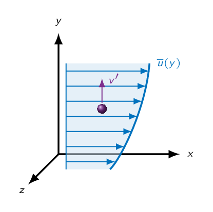
Let's first examine the relation between \(u^\prime\) and \(v^\prime\) (the velocity fluctuations in the \(x\) and \(y\) directions). A fluid particle in a boundary layer (see figure below) will be influenced by the fluctuating velocity. A positive \(v^\prime\) fluctuation will lead to a vertical transport of the fluid particle. The fluid particle will end up in a position in the flow where the axial velocity is higher than where it came from, thus leading to a negative fluctuation in the axial velocity at that position \((u^\prime < 0)\). In the same way, a negative \(v^\prime\) fluctuation will lead to \(u^\prime > 0\). The product \(u^\prime v^\prime\) will always be negative if \(\partial \overline{u}/\partial y\) in the wall-normal direction. Thus \(\tau_{turb}=-\rho \overline{u^\prime v^\prime}=\mu_t \dfrac{\partial \overline{u}}{\partial y}\) is positive.
Prandtl's mixing length conceptIf the fluid particle in the figure below moves the distance \(l_m\) (the mixing length) up or down in the boundary layer, the velocity can be estimated to be. $$\overline{u}(y+l_m)=\overline{u}(y)+l_m\frac{\partial \overline{u}}{\partial y}$$ $$\overline{u}(y-l_m)=\overline{u}(y)-l_m\frac{\partial \overline{u}}{\partial y}$$
The average distance that a small mass of fluid will travel before it exchanges its momentum with another mass of fluid
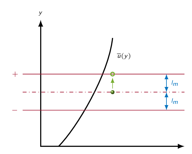
Prandtl assumed that
$$u^\prime\approx l_m\frac{\partial \overline{u}}{\partial y}$$Furthermore, he assumed \(v^\prime\) to be of the same size as \(u^\prime\)
$$\tau_{t}=-\rho\overline{u^\prime v^\prime}\approx\rho l_m^2\left(\frac{\partial \overline{u}}{\partial y}\right)^2$$ $$-\rho\overline{u^\prime v^\prime}\approx\mu_t\frac{\partial \overline{u}}{\partial y}\Rightarrow\mu_t\approx\rho l_m^2\left|\frac{\partial \overline{u}}{\partial y}\right|$$ $$\nu_t=\frac{\mu_t}{\rho}\approx l_m^2\left|\frac{\partial \overline{u}}{\partial y}\right|$$So, how do we estimate the mixing length \(l_m\)? Theodore von Kármán postulated the mixing length to be
$$l_m=\kappa y$$where \(\kappa\) is the von Kármán constant.
$$\mu_t\approx\rho l_m^2\left|\frac{\partial \overline{u}}{\partial y}\right|=\rho \kappa^2 y^2 \left|\frac{\partial \overline{u}}{\partial y}\right| $$ $$\tau_w=\mu_t \frac{\partial \overline{u}}{\partial y} = \rho \kappa^2 y^2 \left(\frac{\partial \overline{u}}{\partial y}\right)^2=\rho {u^{\ast}}^2$$ $$\kappa^2 y^2 \left(\frac{\partial \overline{u}}{\partial y}\right)^2={u^{\ast}}^2\Rightarrow \frac{\partial \overline{u}}{\partial y}=\frac{u^{\ast}}{\kappa y}$$ $$\overline{u}(y)=\dfrac{u^{\ast}}{\kappa}\ln (y)+C$$or in non-dimensional form
$$\underbrace{\dfrac{\overline{u}(y)}{u^{\ast}}}_{u^+}=\dfrac{1}{\kappa}\ln \underbrace{\left(\dfrac{y u^{\ast}}{\nu}\right)}_{y^+}+\underbrace{\dfrac{C}{u^{\ast}}-\ln\left(\dfrac{u^{\ast}}{\nu}\right)}_{B}$$The log law:
$$u^+=\frac{1}{\kappa} \ln \left( y^+ \right) + B$$ where \(\kappa\approx 0.41\) and \(4.9 < B < 5.5\). The log-law is valid for \(30 \lesssim y^+ \lesssim 1000\).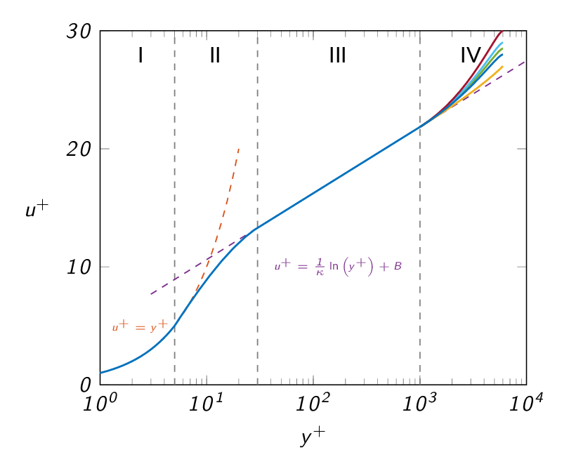
Turbulent Pipe Flow
As we did for laminar pipe flow, we will now obtain the friction factor for turbulent pipe flow
$$\tau_w=f_D\frac{\rho V^2}{8}=\rho {u^\ast}^2\Rightarrow f_D=8\left(\frac{V}{u^\ast}\right)^{-2}$$So, what we need now is an estimate of the average flow velocity in the pipe.
- Assume that we can use the log-law all the way across the pipe
- Integrate to get the average velocity
- Insert the calculated average velocity into the relation above
with \(\kappa=0.41\) and \(B=5.0\) we get
$$\frac{V}{u^\ast}\approx 2.44 \ln \frac{Ru^\ast}{\nu}+1.34$$The argument of the logarithm can be rewritten as
$$\frac{Ru^\ast}{\nu}=\frac{VD}{2\nu}\frac{u^\ast}{V}=\left\{Re_D=\dfrac{VD}{\nu},\ f_D=8\left(\frac{u^\ast}{V}\right)^2\right\}=\frac{1}{2}Re_D\left(\frac{f_D}{8}\right)^{1/2}$$and thus:
$$\frac{1}{\sqrt{f_D}}\approx 2.0 \log_{10} (Re_D \sqrt{f_D})-0.8$$Wall Roughness and Friction
Effects of surface roughness on friction:
- Negligible for laminar pipe flow
- Significant for turbulent flow
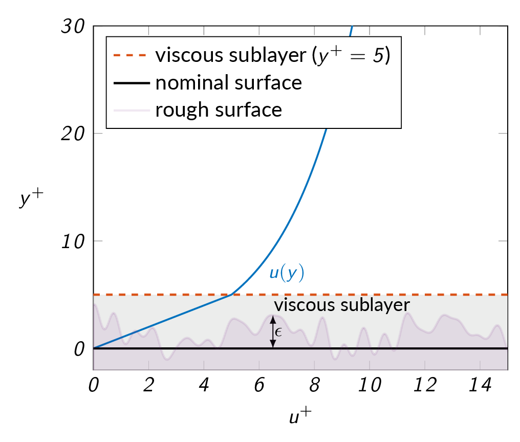
- breaks up the viscous sublayer
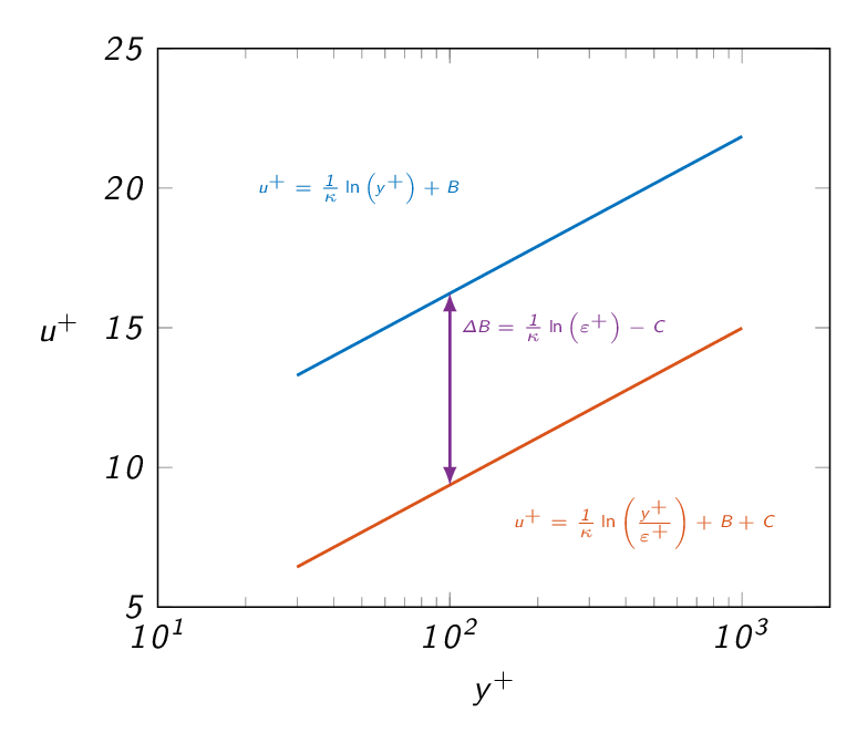
- modifies the log law (changes the value of the integration constant \(B\))
- \(\Delta B\propto (1/\kappa)\ln \epsilon^+\) where \(\epsilon^+=\frac{\epsilon u^\ast}{\nu}\)
- \(\dfrac{\epsilon u^\ast}{\nu} < 5\)
- hydraulically smooth
- no effects of roughness
- \(5 \le \dfrac{\epsilon u^\ast}{\nu} \le 70\)
- transitional
- moderate Reynolds number effects
- \(\dfrac{\epsilon u^\ast}{\nu} > 70\)
- fully rough
- sublayer totally broken up
- independent of Reynolds number
The Colebrook relation below is a combination of theory for perfectly smooth pipes and fully rough pipe flow and forms the basis for the Moody chart presented in the figure below.
$$\frac{1}{\sqrt{f_D}}=-2.0 \log_{10} \left(\frac{\epsilon / D}{3.7}+\frac{2.5}{Re_D \sqrt{f_D}}\right)$$
The grayed area in the Moody chart represent the range of Reynolds numbers where we will have transition from laminar to turbulent flow. SInce there are no reliable models for this specific area, it should in general be avoided.
Study Guide
The questions below are intended as a "study guide" and may be helpful when reading the text book.
- How do we usually define the Reynolds number for pipe flows?
- What does critical Reynolds number mean for a pipe flow?
- What does entrance length mean? How is the flow velocity profile changed during the entrance length?
- What does fully developed pipe flow mean?
- Give three examples of sources of local losses in a pipe system
- Start from Bernoulli's extended equation and the momentum equation for a pipe with the length \(L\) and diameter \(D=2R\) and show that $$\Delta p_f=2\tau_w\dfrac{L}{R}$$
- The Darcy friction factor is defined as $$f=\dfrac{8\tau_w}{\rho V^2}$$ Rewrite the friction loss from the previous question using the Darcy friction factor
- For laminar pipe flows, show that: $$f=\dfrac{64}{Re_D}$$
- What parameters effects the magnitude of \(f\)?
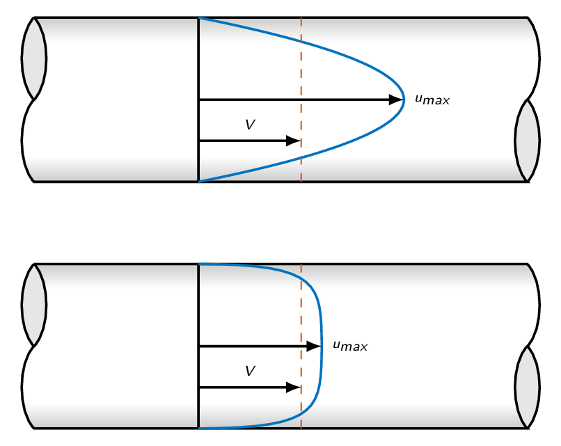
- For fully developed laminar pipe flow, the velocity profile can be expressed as $$u=u_{max}\left(1-\dfrac{r^2}{R^2}\right)$$ Show that the average velocity in fully developed laminar pipe flow is half the maximum velocity.
- Compare the velocity profiles for fully developed laminar and turbulent flow, which of the flows gives the highest wall shear stress for a given mass flow?
- For fully developed turbulent pipe flow, the mean velocity profile can be approximated using the 1/7-rule $$u=u_{max}\left(\dfrac{r}{R}\right)^{1/7}$$ Why should this not be used directly for the calculation of wall shear stress?
- Give three characteristics of turbulent flow
- Turbulent flow is dissipative. What does that mean?
- What defines the largest and smallest length scales in a turbulent flow?
- Explain the concept of Reynolds decomposition
- Why do one often want to use time-averaged equations when studying turbulent flow while that is not the case for laminar flows?
- Explain the closure problem related to the Reynolds-averaged flow equations
- In the Reynolds decomposition, the velocity components and pressure are divided into an average part and a fluctuating part as for example $$u=\bar{u}+u'$$ Define the time average and show that the time average of the fluctuating component is identically equal to zero.
- How is the intensity of the fluctuating velocity component specified?
- Derive the continuity equation for the time-averaged velocity field for incompressible turbulent flow starting from the general continuity equation on differential form $$\dfrac{\partial \rho}{\partial t}+\dfrac{\partial\left(\rho u\right)}{\partial x}+\dfrac{\partial\left(\rho v\right)}{\partial y}+\dfrac{\partial\left(\rho w\right)}{\partial z}$$
- Derive the \(x\)-component of the Navier-Stokes equation for turbulent flow. Explain the physical meaning of each of the terms in the equation.
- Show that the term \(-\rho \overline{u'v'}\) can be interpreted as a shear stress
- How can the turbulent shear stress be related to the mean flow using the turbulence viscosity \(\mu_t\)? What is this assumption called?
- Define the friction velocity \(u^\ast\)
- Derive the average velocity distribution in the viscous sublayer starting from $$\overline{u}\dfrac{\partial \overline{u}}{\partial x}+\overline{v}\dfrac{\partial \overline{v}}{\partial y}=\dfrac{1}{\rho}\dfrac{\partial \tau}{\partial y}$$
- How does the turbulence viscosity \(\mu_t\) compare to the fluid viscosity \(\mu\) in the viscous sublayer and in the fully turbulent region, respectively?
- How does the total shear stress vary with distance from the wall in the viscous sublayer and in the fully turbulent region, respectively?
- How are the velocity profiles characterized mathematically in the viscous sublayer and in the fully turbulent region, respectively?
- Make a schematic representation of the non-dimensional velocity \(u^+\) as a function of the non-dimensional wall distance \(y^+\) for a turbulent boundary layer. The velocity profile can be divided into different regions. Name these regions.
- What relation for the local average velocity is used for the derivation of the friction factor \(f\) for turbulent pipe flow?
- The Moody chart is an engineering tool that can be used for estimation of pressure losses in a pipe flow
- Why does the Moody chart not give reliable values in the Reynolds number range \(2000 < Re < 4000\)?
- How does \(f\) vary with the Reynolds number in the fully turbulent regime?
- What is the effect of surface roughness on the friction factor?
- What can we say about the Moody chart when it comes to accuracy?
- How is the hydraulic diameter defined and how can it be used for calculation of the friction factor \(f\) for laminar and turbulent flow in non-circular ducts?
- Define the loss coefficient \(K\)
| Document Archive | ||
| MTF053_C06.pdf | Lecture notes chapter 6 | |
| MTF053_Turbulence.pdf | Complementary material - Turbulent flow theory | |
| MTF053_Formulas-Tables-and-Graphs.pdf | A collection of formulas, tables, and graphs | |
| MTF053_Study-Guide.pdf | A collection of theory questions that give a good representation of the theory covered in the course | |